The Small Dip Produced by a Planetary Transit

For most of a graph, a star's measured brightness seems ordinary. Then the line falls slightly, stays low for a while, and returns. The dip is small enough that a casual reader might overlook it. Yet this kind of observation can help reveal a world that the telescope does not resolve as a separate point. The exciting part is not that a line moved downward. It is that a carefully tested explanation can connect that movement to an object crossing in front of a distant star.

NASA describes a planetary transit as a planet passing between its star and the observer, temporarily reducing the received starlight.[1] A light curve records brightness over time. It gives us an indirect observation: how much light reached the instrument, and when. To infer a planet, we must establish that a transit model accounts for the pattern and examine alternatives that could produce a similar signal. The small dip is the beginning of the investigation, not its conclusion.

We can follow that reasoning with constructed examples. The stars and planets below are imaginary; their sizes, brightnesses, periods, and noise levels are chosen for transparent arithmetic. No figure is a telescope measurement or a newly discovered object. This lets us separate what a simplified transit model predicts from what a real discovery would require. It also exposes several assumptions that can disappear when a striking light curve is presented without the supporting analysis.

Start with the area that disappears

Imagine a star whose apparent disk has uniform brightness. Put a completely dark, opaque planet in front of it, entirely inside the disk during the middle of the transit. If the planet's radius is one tenth of the star's radius, its projected area is one hundredth of the star's area. Under these assumptions, the received light drops by one percent. The radius ratio is squared because the comparison is between areas. A small change in radius can therefore produce a much larger proportional change in transit depth.

For this ideal full-overlap case, fractional depth equals the square of the planet-to-star radius ratio. A radius ratio of 0.05 produces a depth of 0.0025, or 0.25 percent. A ratio of 0.01 produces 0.0001, or one hundred parts per million. These are three calculations in the same model. They do not establish how easily an instrument will detect any of the signals, because detectability also depends on the observations and other sources of variation.

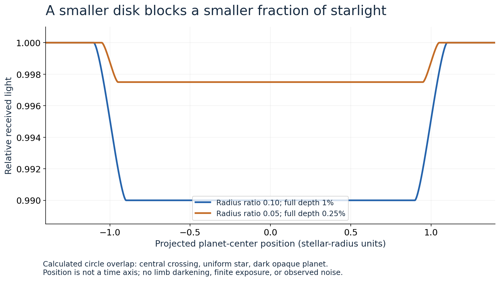
Figure 1. Exact circle-overlap calculation for a uniform stellar disk and a central, straight projected crossing. The horizontal axis is the planet center's projected position in stellar-radius units, not elapsed time. No atmospheric emission, limb darkening, or observed noise is included.

The inverse calculation is just as revealing. Suppose the measured depth is one percent and the model applies. Taking the square root gives a planet-to-star radius ratio of 0.1. That is a relative size. To obtain an absolute planetary radius, we also need the stellar radius. If the star's radius is assumed to be 700,000 kilometres, the planet's becomes 70,000. If the stellar radius is revised upward by twenty percent while the ratio stays fixed, the inferred planetary radius increases by twenty percent too.

The star is therefore part of the measurement. A precise light curve does not make uncertainty in the stellar radius disappear. Nor does the depth alone provide the planet's mass. Two objects with the same projected radius can have different masses and compositions. I would keep those quantities separate when reading a discovery account: which properties come from the transit, which come from additional observations, and which come from a model that combines them?

The edges contain information too

Our simple area ratio applies while the planet's disk is fully in front of a uniformly bright star. During entry and exit, the projected disks overlap only partly. The brightness changes as that overlap grows and shrinks. A path across the center and a path nearer the edge can therefore have different shapes and durations. A grazing passage can avoid the full-overlap situation entirely. Reading one minimum value without the surrounding curve throws away information that may help constrain the geometry.

Real stellar disks are not generally uniform in apparent brightness. Mandel and Agol's 2002 paper develops analytic transit light curves with limb darkening, accounting for variation across the stellar disk.[2] That physical structure changes the shape of the dip. The paper is a useful reminder that a plotted transit model is not merely a box placed under a noisy line. Its shape connects geometry and a description of the light source. The model's assumptions matter when extracting precise parameters.

For an intuitive constructed comparison, imagine blocking equal small areas near the center and near the edge of a star whose center appears brighter. The areas match, but the blocked light need not. Our original area-only argument would no longer describe both positions correctly. The correction is not an arbitrary adjustment to rescue the planet hypothesis; it is a prediction of the stated brightness distribution. The investigator should choose and test that distribution using the relevant stellar and observational information.

Exposure duration creates another layer. Suppose a measurement averages the light collected over thirty minutes while the entry phase lasts ten minutes. The recorded point blends different overlap states. It cannot be interpreted as an instantaneous sample without accounting for that averaging. This is an invented timing example, but the principle is straightforward: the instrument measures over an interval, while a model may initially describe a value at an instant. Comparing them requires the same observation rule on both sides.

Repetition makes a stronger question

Now imagine similar dips separated by ten days. The repetition suggests a candidate orbital period, provided the events belong to the same process. It also creates a prediction: another dip should occur near a calculable time. Observing that event with appropriate coverage adds evidence. But regularity alone does not identify the transiting object as a planet. Other recurring phenomena can produce changing brightness. The timing must be considered alongside the depth, shape, source location, and independent constraints.

The observing window can make periods ambiguous. Suppose recorded dips occur on days zero and twenty, while no usable observations exist around day ten. A twenty-day period fits the two events, but a ten-day period with a missed transit can fit as well. The absence of data around the intermediate prediction cannot be treated as absence of a transit. A useful follow-up targets times where the competing period hypotheses differ. This turns uncertainty into an observing question rather than a reason to select the more attractive number.

For another simple calculation, assume a three-hour transit every ten days. Ten days contain 240 hours, so the star is in transit for 1.25 percent of that interval. An observation covering a randomly chosen brief interval may miss the event even if the planet exists. The exact detection probability requires the sampling schedule and geometry, but the duty-cycle calculation already warns against reading a short flat light curve as strong evidence of no planet. Coverage and sensitivity must accompany a nondetection.

Combining repeated events can reveal a weak pattern. If a trial period is correct, aligning observations by orbital phase can place corresponding portions of several transits together. But that alignment is an analysis choice. I would inspect the individual events as well as the combined curve. One unusually strong dip or a processing artifact can influence a tidy average. A persuasive presentation shows that the repeated evidence supports the interpretation rather than asking the reader to trust only the smoothest final panel.

A neighboring star changes the arithmetic

Suppose the target star supplies one arbitrary unit of light outside transit. A planet blocks one percent of that star's light, reducing it to 0.99 units. Now add an unresolved companion or background star that contributes another one unit and does not dim. The instrument records a baseline of two units and an in-transit total of 1.99. Relative to the combined baseline, the observed dip is only half a percent. The planet has not changed size. The light used as the denominator has changed.

If an analyst incorrectly treats all that light as coming from the host star, the simple radius-ratio estimate becomes the square root of 0.005, approximately 0.0707. The true stipulated ratio is 0.1. Correcting the equal-brightness dilution increases the inferred ratio by a factor of about 1.414. This is an original calculation, not a claim about a particular observed system. It demonstrates why identifying which light belongs to which star matters before assigning a size to the planet.

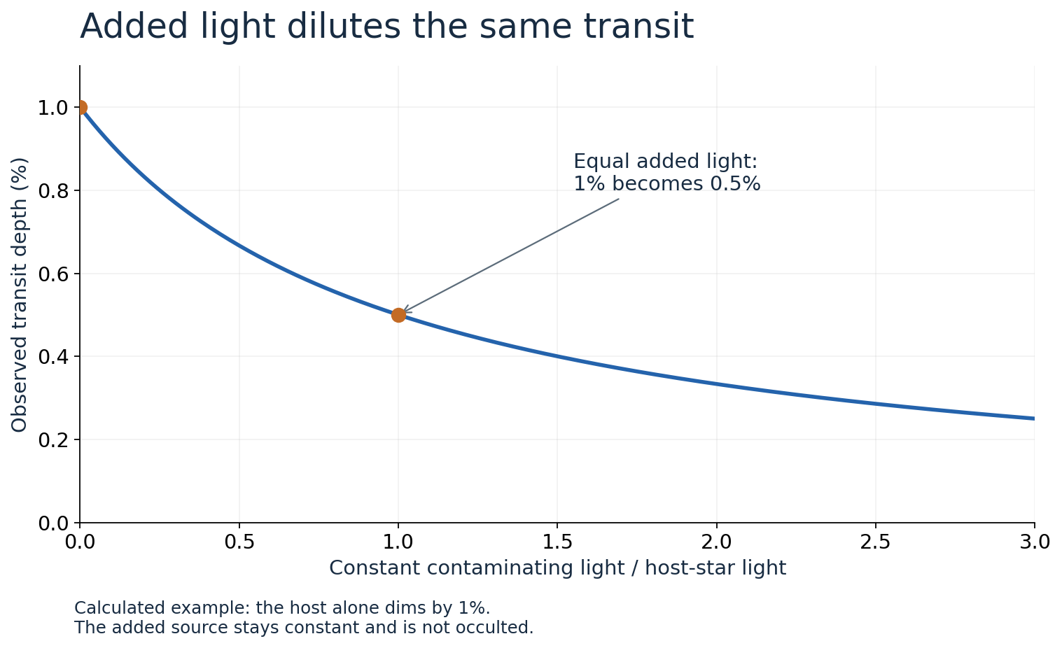
Figure 2. Calculated dilution: observed depth = host-only depth / (1 + contaminating-light ratio). The added light is assumed constant and unocculted. At an equal contribution from another source, one percent becomes half a percent.

NASA JPL's account of research on stellar companions describes this dilution problem and its consequences for inferred planetary radii.[3] The practical lesson is larger than one numerical correction. The aperture used to collect light may contain contributions from more than one object, and determining the actual host matters. An apparently small transit can reflect a small occulting object, diluted light from a larger eclipse, or another configuration. Additional observations help distinguish those possibilities.

A useful thought experiment asks what happens if we change the measurement aperture while accounting for the instrument's response. If including more of a nearby source changes the apparent dip as predicted by a blending hypothesis, that relationship deserves investigation. It is not a universal test with an automatic answer: changing an aperture can change noise and systematic effects too. The point is to make the competing explanations predict different observations, then evaluate those observations with the relevant measurement model.

A real false-positive investigation

The possibility of a misleading dip is not an objection invented after a discovery. It is part of the research method. Torres and colleagues' study of Kepler-9 modeled blended configurations, including eclipsing systems whose light is diluted by other stars, and combined that modeling with follow-up constraints.[4] Their BLENDER approach examined whether alternatives could reproduce the observations. The work illustrates why identifying a planet can require actively testing other explanations rather than simply fitting a planetary transit curve.

A model that fits well is necessary evidence for an explanation, but it may not be exclusive evidence. In our constructed dilution example, different combinations of source brightness and eclipse depth can produce the same observed fractional drop. One number cannot distinguish all those combinations. Additional information about the sources can reduce the ambiguity. This is an inverse problem: several physical scenes may map into similar measurements, so a convincing inference needs observations that separate the scenes.

NASA's archive also describes the Kepler Data Validation work by Twicken and colleagues, which applied diagnostic tests to candidates to help distinguish transiting planets from instrumental and astrophysical false positives.[5] Detection and validation are different stages. Finding a pattern that crosses a search threshold creates something to examine. It does not make every later question disappear. A discovery account becomes more informative when it tells the reader which tests the candidate survived and which limitations remain.

For a fictional candidate, I would organize those questions around concrete alternatives. Could the dip arise from a different object contributing light? Does the same feature appear in unrelated targets at the same time? Does it remain when reasonable processing choices change? Is its timing consistent across individual events? These are investigative questions, not a substitute for a mission's validated pipeline. Their value is to connect each doubt with evidence that could strengthen or weaken it.

How small is small compared with the noise?

Return to a hypothetical depth of one hundred parts per million. Assume individual measurements have independent, zero-mean noise with standard deviation two hundred parts per million, and that the out-of-transit baseline is known exactly for this exercise. Averaging one hundred comparable in-transit measurements reduces the noise standard deviation of their mean to twenty parts per million. Under those assumptions, a one-hundred-part-per-million depth is five times that standard deviation. The improvement follows from averaging independent observations.

That arithmetic does not establish a discovery significance for a real search. The baseline is not generally known exactly, noise can be correlated, and searching many possible periods and durations changes the statistical question. The calculation isolates one contribution to sensitivity. It would be misleading to quote the resulting factor of five while silently dropping the assumptions. I would want the actual analysis to include the observation process and the range of hypotheses that were searched, not just the most favorable average.

Consider a counterexample with a slowly drifting instrument baseline. If neighboring points share the same drift, taking more points in the same short interval does not provide as many independent measurements as the square-root rule assumes. Their agreement can reflect the shared disturbance. Repeated transits observed under different conditions may supply more useful evidence than many closely spaced samples of one event, depending on the disturbance. The structure of the noise matters as much as its single-point amplitude.

An analysis also has to decide which variations to remove. Suppose an overly flexible baseline model is allowed to bend through a shallow dip. It may absorb part of the signal we intended to measure. Conversely, a poor baseline model might leave a residual that resembles a transit. These are constructed possibilities, but they motivate a practical check: apply the full processing method to known injected signals and assess what it recovers. A clean final graph is not enough to establish that the processing preserved the relevant depth and shape.

Test the pipeline with something whose answer is known

An injection-and-recovery exercise begins by adding a specified synthetic signal to suitable data or a simulated measurement stream, then running the analysis without giving it the answer. In our teaching example, choose the depth, period, duration, and observation times explicitly. Compare the recovered values with the injected ones. The exercise can reveal missed signals or biased estimates under those conditions. It cannot prove that every unknown real-world disturbance is represented in the test.

The location of the injection matters. Adding a dip to an already corrected light curve tests only the processing after that point. It does not test earlier image calibration or light extraction. Adding a model earlier in the chain can address more stages, provided the synthetic signal is constructed appropriately. I would describe the injection point in any reported performance result. Otherwise a successful partial test can be mistaken for evidence about the entire measurement pipeline.

We should test nondetections too. A procedure that recovers every inserted dip while also reporting many spurious ones has a different value from one that distinguishes them reliably. The threshold trades sensitivity against false alarms, and the relevant rates depend on the tested population and conditions. A useful evaluation reports what was searched and what counted as a correct match. Simply showing several recovered examples can be persuasive without revealing how often the method was wrong elsewhere.

For the imaginary ten-day candidate, a follow-up observation has a more direct role. Use the fitted timing to predict a future transit window, account for uncertainty, and ask whether the expected feature appears in adequate data. If it does, compare its shape and depth with the prior events. If it does not, first establish whether the coverage and sensitivity were sufficient to test the prediction. A missed window and a well-observed absent event have different implications for the hypothesis.

What the dip does not tell us by itself

A radius estimate is not a photograph of a surface. It does not independently reveal oceans, weather, a solid composition, or life. Those claims would require additional observations and models appropriate to each question. The transit is already an impressive piece of evidence without attaching every interesting planetary property to it. I would rather know exactly what was measured than receive a richer description whose most memorable details came from assumptions the data did not test.

The same restraint applies to an illustration. A colorful artist's planet can help readers imagine scale or context, but it should not be confused with a resolved image of the object. Our figures use calculated curves instead because the relevant evidence is a change in received light and the geometry that could produce it. The distinction should remain visible in a public article. Otherwise the picture can make an uncertain physical description feel observed before the text has even begun.

The observing geometry also limits what a transit survey sees. A planet whose orbit never carries it across the stellar disk from our viewpoint will not produce the dip described here. A survey's list of detected transits is therefore shaped by alignment as well as instrument sensitivity and observing time. Inferring the wider population requires accounting for that selection. Counting the objects found is an observation; estimating how many exist beyond the observed sample is an additional analysis.

A small signal can support a large conclusion

For our ideal example, the path from dip to size is explicit: define a uniform stellar disk, measure a fractional loss, take its square root to obtain a radius ratio, and supply an independently constrained stellar radius. Each additional realism changes something that must be modeled or measured: limb darkening, partial overlap, exposure averaging, contaminating light, and noise. The result can remain powerful, but it becomes powerful through those checks rather than by ignoring their complexity.

A useful account of a real candidate should make the evidence chain similarly visible. It should show the light curve and observation conditions, explain the transit fit, describe the tests against alternatives, and distinguish measured quantities from inferred properties. Uncertainty should accompany the parameters it affects. Readers can then understand why the result deserves confidence and what future observations could improve or challenge. A single dramatic dip deserves curiosity; a coherent body of evidence deserves a stronger conclusion.

The most interesting thing about transit science is that so little light can carry so much information when the question is carefully framed. The telescope does not hand us a named world with its properties attached. It supplies measurements from which several explanations are possible. By predicting, comparing, and eliminating alternatives, an investigation can connect a small loss of starlight to an orbiting planet. The size of that conclusion is earned by the method, not by the depth of the dip alone.

References and method

1. NASA Science, What's a Transit?; transit geometry and light curves.
2. Kaisey Mandel and Eric Agol, Analytic Lightcurves for Planetary Transit Searches, 2002; uniform-source geometry and limb-darkened transit models.
3. NASA JPL, Hidden Stars May Make Planets Appear Smaller, 2017; dilution by stellar companions.
4. Guillermo Torres and colleagues, Modeling Kepler Transit Light Curves as False Positives: Rejection of Blend Scenarios for Kepler-9, and Validation of Kepler-9 d, 2011; modeling alternatives with follow-up constraints.
5. Joseph D. Twicken and colleagues, Kepler Data Validation I: Architecture, Diagnostic Tests, and Data Products for Vetting Transiting Planet Candidates, 2018; candidate diagnostics and data products.

All numerical stars, planets, observing schedules, and noise examples are constructed. Figures are calculated illustrations and do not represent discoveries or observed light curves. Sources checked on 3 October 2026.

Explore the complete Signals Around Us series.