How a Neuronal Signal Begins

A neuron fires. The phrase makes the event sound instantaneous, almost like a software instruction changing a bit. On a recording, there is a sharp excursion that can be marked with one timestamp. But immediately before that mark, the cell was already doing something: currents were flowing, membrane voltage was changing, and the state of ion channels was evolving. The discrete event is useful for analysis. It is not the whole physical process that produced the event.

For someone used to electronic and communication systems, the temptation is to identify a wire, a threshold, and a pulse, then treat the analogy as a complete explanation. I find the analogy more useful when we investigate where it stops working. A neuron is a living electrochemical system. Its behavior depends on membrane properties, ionic gradients, channel dynamics, geometry, and history. A compact model can explain one relationship while leaving most of that machinery out.

This article follows a deliberately simple membrane calculation and compares its assumptions with the experimental tradition established by Hodgkin and Huxley. Their 1952 work described currents and excitation in the squid giant axon using a quantitative conductance model.[1] Our numerical examples are teaching models, not recordings from that experiment or predictions about a person's brain. The aim is to understand how a signal can emerge from changing physical conditions before asking what that signal means to a larger circuit.

Voltage is a difference across a membrane

Membrane potential describes an electrical potential difference between the inside and outside of a cell. A negative value means the inside is at a lower potential than the chosen outside reference. It does not mean the cell contains only negative charge or that ions have stopped moving. The membrane separates regions with different ionic conditions, and selective pathways allow currents to flow. A voltage measurement summarizes part of that state; it does not enumerate every molecule or every process maintaining it.

For our constructed example, choose a resting reference of minus seventy millivolts. This is a model parameter, not a universal resting value for every neuron. Moving to minus sixty millivolts is a ten-millivolt depolarization relative to that starting point. The number becomes less negative. This elementary sign convention matters because an explanation can become confusing when it alternates casually between “more voltage,” “more negative,” and “more activity” without stating the direction or the measured quantity.

I would also ask where and how the voltage was measured. A recording across the membrane of one cell and an extracellular recording near several cells are different observations. A large waveform on one instrument does not directly equal a large membrane potential in another measurement arrangement. The electrode, reference, geometry, and acquisition chain contribute to the recorded signal. Before drawing a circuit analogy, identify which physical difference the ordinate actually represents.

A membrane can store charge and allow current to leak

One useful approximation represents the membrane with a capacitance and a leak pathway. Capacitance relates stored charge to voltage difference. Resistance describes the relationship between voltage and current through the simplified leak. This circuit does not contain all the voltage-dependent channels needed to reproduce a real action potential. It can still show why an input does not necessarily produce an instantaneous voltage change and why the recent history of inputs can matter.

Choose a capacitance of two hundred picofarads and a resistance of one hundred megohms. Their product is twenty milliseconds, the time constant of our linear model. For a step of constant input current, voltage approaches a new steady level exponentially. After one time constant, it has completed approximately 63.2 percent of the eventual change. That percentage follows from the exponential function; it is not a measured property claimed for all neurons or all experimental conditions.

An input of two hundred picoamperes multiplied by one hundred megohms gives a steady voltage change of twenty millivolts. Starting from minus seventy, the passive model approaches minus fifty millivolts. It does not jump there immediately. In the compact expression V(t) = Vrest + RI(1 − exp(−t/RC)), each symbol has a physical role and unit. The equation is useful because its assumptions are visible enough to calculate and challenge.

A threshold model can predict an event without modeling its shape

Add a chosen threshold of minus fifty-five millivolts. The model needs to rise fifteen millivolts from its starting point before we register an event. Under the two-hundred-picoampere step, that is three quarters of the eventual twenty-millivolt rise. Solving the exponential gives a first crossing after approximately 27.7 milliseconds. This is the event time of our stipulated threshold model. It is not a universal neuronal latency or a claim that all membranes have that threshold.

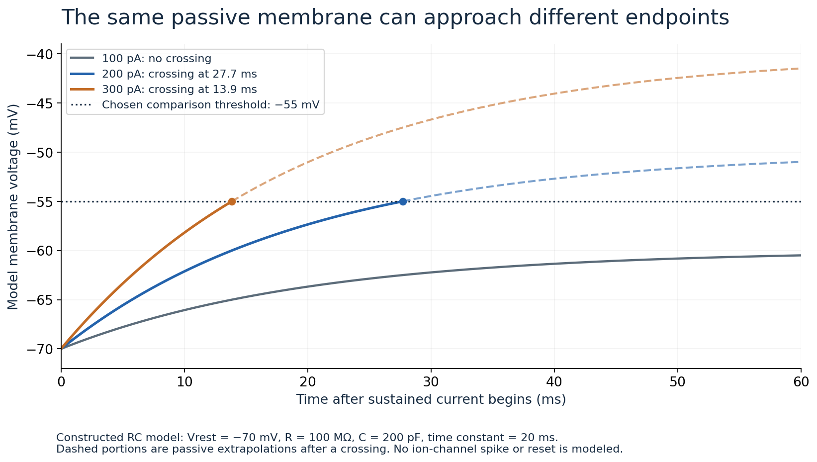
Figure 1. Constructed passive model: resting reference −70 mV, resistance 100 MΩ, capacitance 200 pF, and chosen threshold −55 mV. Dashed continuations after a crossing are passive extrapolations. The figure does not simulate an action-potential waveform or a biological reset.

Reduce the current to one hundred picoamperes. The eventual rise is only ten millivolts, so voltage approaches minus sixty and never reaches the chosen threshold in this model. Increase current to three hundred picoamperes and the eventual rise becomes thirty millivolts. Reaching the same fifteen-millivolt threshold difference now requires half the final rise, giving approximately 13.9 milliseconds. The comparison exposes how both input magnitude and the membrane's integration timescale affect the first event.

Allen Institute documentation describes generalized leaky integrate-and-fire models that evolve voltage, track thresholds, and apply reset rules when an event is registered.[2] That is a family of modeling choices, with different levels of complexity. Our example is simpler still: it calculates passive charging up to an imposed criterion. A model can be useful for predicting selected event times while omitting the ionic mechanism and detailed shape of the spike. Its usefulness does not erase that omission.

An action potential needs regenerative dynamics

The rapid rise of an action potential cannot be explained by our fixed leak and capacitance alone. In the classic axon account, voltage-dependent sodium and potassium conductances change over time. Depolarization can increase inward sodium current, which further changes voltage and channel state; subsequent changes, including sodium inactivation and potassium conductance, contribute to the return toward lower voltage. Hodgkin and Huxley's model links these interacting dynamics quantitatively.[1] It does not reduce the event to a switch with no physical history.

The distinction matters when interpreting a threshold. An algorithm may identify a point on the rising voltage trace as the beginning of a spike. The underlying membrane dynamics need not contain a universal, immutable comparator set to that exact voltage. Channel availability and the trajectory approaching the event can matter. A useful operational definition of threshold should therefore be reported with the method used to estimate it and the conditions of the recording.

The classic study also has a specific experimental scope: squid giant axon, with its preparation, temperatures, measurements, and model parameters. It established a powerful mechanistic framework. It did not imply that one parameter set describes every cell in every nervous system. I would separate the general idea of changing conductances from the quantitative behavior of a particular preparation. That distinction allows the model to teach without turning a landmark experiment into an unsupported universal specification.

Two small inputs can depend on their timing

A second constructed model makes timing visible. Suppose one brief input produces an instantaneous ten-millivolt rise above the resting reference, followed by exponential decay with a twenty-millisecond time constant. The instantaneous rise is an idealization of an input, not a realistic simulation of a synapse. Let two such responses add linearly, with no active channels or reset. We can then ask how the interval between them changes the maximum passive voltage excursion.

If the second input arrives five milliseconds after the first, the remaining contribution from the first is ten times exp(−5/20), about 7.79 millivolts. Adding the new ten gives a 17.79-millivolt excursion. Against our chosen fifteen-millivolt threshold difference, the sum crosses the criterion. If the second arrives thirty milliseconds later, only about 2.23 millivolts remain from the first. The combined excursion is 12.23 millivolts and stays below that same criterion.

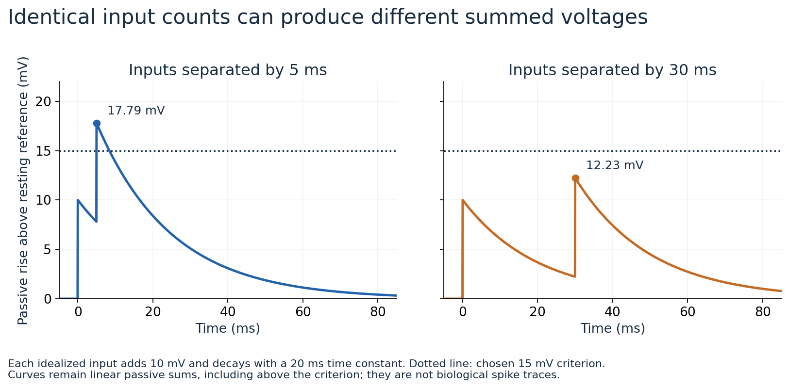
Figure 2. The linear toy model sums two 10 mV exponential responses with a 20 ms time constant. Close timing produces 17.79 mV at the second input; wider separation produces 12.23 mV. Curves remain passive sums even above the reference line; no action potential is simulated.

The number of inputs and the size of each are identical in the two cases. Their timing differs. That is enough to change the result in this model. A count that discards the interval would miss the distinction. Real synapses and dendrites introduce additional conductance, spatial, and nonlinear effects, so the simple sum should not be treated as a complete neuron. It establishes one narrower lesson: an event can depend on temporal arrangement, not only on how many inputs occurred.

Location changes what an input can do

Our calculation places every input into one shared compartment. A real neuron has spatial structure, so that simplification can conceal important differences between inputs at different locations. A signal arriving on one branch need not affect the spike-initiation region in the same way as an otherwise similar signal arriving elsewhere. The membrane and internal pathways form a distributed system. The single-compartment model removes that geometry intentionally so we can inspect one temporal relationship clearly.

For an engineering analogy, consider two sensors connected through different filters to one decision stage. Equal sensor outputs do not guarantee equal effects at the decision stage if the intervening paths differ. The analogy helps explain why the input's location belongs in the model, but it does not identify the biological transfer function. That requires appropriate measurements or a more detailed model. Borrowing a familiar systems concept is useful only while its scope remains explicit.

Allen's Cell Types resources provide morphology information as well as electrophysiological recordings and computed features.[3] That separation is useful evidence of the kinds of data a richer investigation may require. A voltage trace, a reconstruction of cellular shape, and a fitted model answer different questions. Combining them can support a stronger explanation, but the combination still needs a clear account of which observations constrain which parameters and which conclusions remain predictions.

The stimulus and the response must be kept together

Imagine receiving a voltage trace without the current that was applied during the experiment. You can describe its peaks and intervals, but the missing stimulus limits what you can infer about responsiveness. A delayed spike might reflect the timing of the input rather than an intrinsic delay in the cell. A quiet segment might reflect absent stimulation. The input history is not supplementary decoration; it is part of the evidence needed to interpret the observed dynamics.

The AllenSDK Cell Types example explicitly retrieves the injected-current stimulus and voltage response for a sweep, with their sampling rate and units.[3] It also demonstrates extracting features such as threshold and width. Those operations provide a useful distinction between the recorded waveforms and the quantities computed from them. A feature table is a derived representation. Another algorithm or preprocessing choice may produce a different feature estimate without changing the original recorded samples.

I would preserve the raw or appropriately documented source recordings, stimulus timing, units, preprocessing, and feature definitions together. If a proposed finding concerns spike onset, check whether filtering shifts or smooths the relevant rise. If it concerns amplitude, check calibration and clipping. If it concerns a missing spike, inspect detection criteria and the underlying trace. The analysis should be able to return from the summary table to the observation that generated each important claim.

A detected event is not yet an explanation of meaning

Suppose a hypothetical cell produces twenty detected events during one second. The count supports an average rate of twenty events per second over that interval. It does not establish what stimulus, decision, or experience those events represent. Two sequences can share that count while differing sharply in timing. One can contain a brief cluster and a long silence; another can be more evenly spaced. Which distinction matters depends on the receiving circuit and the experimental question.

The same caution applies to an isolated spike. We can investigate how the membrane generated it without knowing its role in a behavior. A mechanistic account at the cellular level and a functional account at the circuit level are connected but distinct. Calling a spike “a thought” skips the evidence needed to connect those levels. I would ask what was manipulated, what was recorded elsewhere, and which alternative explanations the experiment can distinguish before assigning a broad psychological meaning.

This is where the computer metaphor often becomes too confident. A timestamped event resembles a message in a log, but a log entry acquires meaning from a defined system context. Biological context includes connectivity, ongoing activity, and the state of receiving cells. The metaphor is useful for organizing questions about timing and communication. It becomes misleading when it replaces the experimental work required to determine what a particular pattern does in a particular circuit.

Change a parameter and watch the prediction change

Return to the passive charging example and double capacitance from two hundred to four hundred picofarads while keeping resistance and current fixed. The steady twenty-millivolt rise is unchanged because it depends on resistance times current. The time constant doubles to forty milliseconds. Reaching three quarters of the rise now takes approximately 55.5 milliseconds rather than 27.7. This isolates one model relationship: more capacitance slows the approach without changing the final level under those fixed conditions.

Now instead halve resistance to fifty megohms while retaining the original capacitance and two-hundred-picoampere current. The time constant falls to ten milliseconds, but the eventual rise falls to ten millivolts. The voltage responds more quickly toward an endpoint that no longer reaches the chosen threshold. Faster dynamics do not automatically mean easier firing. The result depends on both the timescale and the available voltage excursion, which changed together in this second comparison.

These parameter changes are mathematical experiments on a stated model. They should not be presented as measurements or as simple instructions for changing a biological cell. Their value is explanatory: they reveal what the model predicts if one quantity changes while the others remain fixed. A real experiment may change several properties at once. An observed difference should therefore be interpreted through the actual intervention and measurements, rather than attributed to one convenient parameter by analogy alone.

Follow the charge as an independent calculation

The passive model offers another check on the numbers. Raising a two-hundred-picofarad capacitance by fifteen millivolts requires three picocoulombs of additional charge on the capacitor, using charge equal to capacitance times voltage change. If the entire two-hundred-picoampere input charged that capacitor with no leak, supplying three picocoulombs would take fifteen milliseconds. Our leaky model took approximately 27.7 milliseconds. The difference is expected because an increasing portion of the input flows through the leak pathway as voltage rises.

At the chosen threshold, the fifteen-millivolt displacement across one hundred megohms corresponds to a leak current of one hundred and fifty picoamperes. Of the two-hundred-picoampere input, only fifty remain to increase the capacitor's voltage at that instant in this model. Dividing by two hundred picofarads gives a slope of 0.25 volts per second, or 0.25 millivolts per millisecond. Initially, when the displacement and leak current are zero, the slope is one millivolt per millisecond.

Those two slopes explain why a straight-line extrapolation from the initial rise reaches the threshold too early. Charging slows as the leak contribution grows. The exponential formula and the instantaneous current balance tell the same story in different forms. An independent calculation like this is useful because it can catch a units error or an inappropriate approximation. It also shows that the familiar curved trace represents a changing division of current, rather than a mysterious delay inserted by the equation.

A recording can end before the predicted event

Suppose an experiment on our mathematical model retains only the first twenty milliseconds after the two-hundred-picoampere step. No threshold crossing appears in that record, because the predicted first crossing occurs later, around 27.7 milliseconds. Reporting “no event observed within twenty milliseconds” is accurate. Reporting “this input can never produce an event” would exceed the observation. The difference is about the time boundary of the evidence, not about whether the calculation contains a sharp threshold.

This matters when comparing a genuinely subthreshold model input with one that would produce a later event. The one-hundred-picoampere case never reaches our chosen criterion under a sustained step. The two-hundred-picoampere case does, but not within the truncated window. A table containing only zero detected events could make those responses look identical. Preserving voltage trajectories, input duration, and observation length allows the analysis to distinguish the different explanations for the same count.

The same care applies when stimulation itself ends before a crossing. If the input is removed at twenty milliseconds, the subsequent passive trajectory changes and decays toward the resting reference. We cannot continue using the sustained-step formula as though the current were still present. Model predictions must follow the actual stimulus history. That is a small technical requirement with a large interpretive consequence: a missing event can reflect insufficient amplitude, insufficient duration, or another condition that a count alone does not reveal.

The useful boundary between a model and a cell

A model earns trust by answering a defined question and surviving comparison with relevant evidence. Our leak-and-capacitance calculation explains charging and temporal summation under deliberately restrictive assumptions. A conductance model can address mechanisms it omits. A spatial model can address relationships lost in one compartment. Increasing complexity is valuable when it resolves a concrete mismatch or enables a needed prediction. A larger set of equations is not automatically a better explanation of the particular observation under investigation.

I would report which properties were fitted and which were predicted independently. Matching a trace used to choose parameters is different evidence from predicting a response to a new input. If several parameter combinations reproduce the same observation, the result may not uniquely identify the underlying mechanism. That is a familiar problem in systems engineering as well as biology. The appropriate response is to seek measurements that distinguish the alternatives, not to hide the ambiguity behind a visually convincing curve.

The beginning of a neuronal signal is therefore both simpler and richer than the word “fires” suggests. We can calculate how a chosen current changes a simplified membrane voltage and when an imposed criterion is crossed. To explain a real action potential, we must also account for the changing biological pathways that make the event regenerative. The sharp mark on the graph is useful. Understanding it means following the continuous physical process that made that mark possible.

References and method

1. A. L. Hodgkin and A. F. Huxley, A Quantitative Description of Membrane Current and Its Application to Conduction and Excitation in Nerve, 1952; original squid-axon conductance model. An accessible scan is hosted by Caltech.
2. Allen Institute, Generalized Leaky Integrate-and-Fire Models; modeled voltage, threshold, and reset dynamics.
3. Allen Institute, Cell Types Database Example; stimulus and response recordings, morphology, and computed electrophysiology features.

All plotted voltages and currents are constructed. The figures use passive exponential equations and chosen comparison thresholds; they neither reproduce an action potential nor fit a biological recording. No Allen Institute recording is plotted or claimed as newly analyzed here. Sources checked on 3 October 2026.

Explore the complete Signals Around Us series.