Attenuation and Dispersion: Two Ways an Optical Signal Can Fail

The optical receiver reports a power level inside its permitted range, but the link still produces errors. The first instinct is to distrust the meter or search for a dirty connector. Both may deserve investigation. There is also a more basic possibility: enough optical energy reached the receiver, but it did not arrive in a form the receiver could reliably distinguish. A power reading describes one property of the received signal. Recovering a sequence of decisions requires more than that property alone.

Two mechanisms make the distinction particularly clear. Attenuation reduces optical power between defined points. Dispersion changes the relative arrival times of components of the signal and can spread a pulse. Corning's optical-fibre glossary separates these concepts, and its engineering note explains why both can constrain transmission.[1][2] The mechanisms can coexist, but they do not answer the same question. A successful loss budget does not independently establish that a high-speed waveform will arrive with acceptable timing distortion.

I want to investigate a constructed forty-kilometre link using both kinds of accounting. Every coefficient, component loss, receiver limit, and source width below is chosen for illustration. These are not specifications for a named transceiver or a recommendation to build a particular link. The purpose is to expose what each calculation includes, which assumptions it needs, and why a plausible result from one instrument cannot settle every question about communication through glass.

Start with two endpoints and a wavelength

An attenuation measurement compares power at one boundary with power at another. If a source delivers one milliwatt at the launch boundary and a tenth of a milliwatt reaches the receiving boundary, the loss is ten decibels. A power level in dBm instead compares one measured power with the reference of one milliwatt. The source is zero dBm and the receiver is minus ten dBm. Mixing the loss and the absolute level without identifying their roles is an easy way to corrupt a budget.

The wavelength belongs in the measurement record. A fibre's attenuation coefficient and dispersion behavior depend on wavelength, and the source, receiver, and test instrument must be interpreted at the relevant operating conditions. A measurement made at one wavelength is not automatically a certificate for all others. I would also record which connectors and patch leads lie inside the tested boundary. Otherwise two technically competent people can obtain different losses simply because they have measured different physical paths.

For our model, choose an attenuation coefficient of 0.25 decibels per kilometre at one stated but otherwise unspecified operating wavelength. Across forty kilometres, the distributed fibre loss is ten decibels. That is a linear increase in the logarithmic loss measure, not a linear subtraction of milliwatts with distance. Each additional section applies another power ratio. The distinction explains why a constant decibel loss per kilometre corresponds to exponential power reduction along an ideal uniform fibre.

Follow the light through a complete loss budget

Add four splices, each assigned a hypothetical loss of 0.1 decibel, and two connector pairs, each assigned 0.5 decibel. The modeled path loss is ten plus 0.4 plus one, or 11.4 decibels. Starting from zero dBm, the predicted received level is minus 11.4 dBm. Converting back to linear units gives approximately 0.0724 milliwatts, or 72.4 microwatts. The result is an accounting prediction under the chosen conditions, not a substitute for measuring the installed path.

Suppose the hypothetical receiver's sensitivity is minus eighteen dBm for a specified operating mode and error criterion. The difference between predicted received power and that sensitivity is 6.6 decibels. If the design reserves three decibels for the explicitly chosen margin, the remaining allowance is 3.6 decibels. A margin is not another measured physical loss. It is reserved headroom intended to cover identified uncertainty or future variation within a design argument that should be explained.

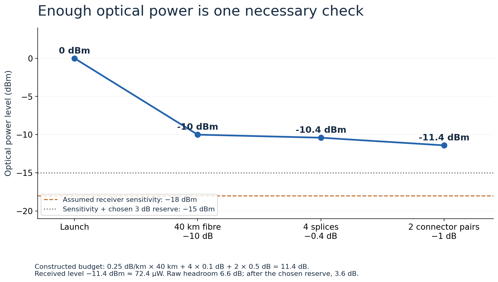
Figure 1. The modeled received power is −11.4 dBm. The assumed sensitivity is −18 dBm, leaving 6.6 dB before reserving 3 dB. All values are illustrative; a real receiver's limits must be taken from its specification for the intended mode and conditions.

The other end of a receiver's permitted range matters too. More power is not an unlimited remedy; a receiver can have a maximum acceptable input as well as a minimum. A complete check uses both limits. I would also distinguish minimum guaranteed launch power from a favorable typical measurement. Combining a typical transmitter value with a worst-case receiver limit can create an optimistic budget whose apparent reserve is less defensible than the arithmetic suggests.

A small decibel change can consume the reserve

Imagine an additional three-decibel loss appears somewhere in our constructed path. The predicted received level falls from minus 11.4 to minus 14.4 dBm, and the optical power is approximately halved. The original 6.6-decibel separation from sensitivity becomes 3.6. After retaining the same three-decibel reserve, only 0.6 decibel remains. The link might still meet the simplified power criterion, but most of its unallocated allowance has disappeared. A small-looking change in a logarithmic number can therefore matter operationally.

That observation does not identify the cause of the extra loss. It could be distributed or concentrated, stable or intermittent, associated with a connection or another part of the path. I would first compare measurements at consistent boundaries and conditions. If a change is real, the next measurement should help localize it. Replacing several components at once might restore service, but it would provide weaker evidence about the original mechanism than a controlled comparison around the suspected section.

Measurement uncertainty also belongs in this reasoning. If two readings differ by a small amount relative to their combined uncertainty and setup variation, the difference should not automatically be treated as physical degradation. Preserve the reference procedure, instrument settings, connection state, and repeatability. A budget reported to two decimal places can still rest on components whose behavior is known much less precisely. Extra digits do not create extra knowledge about the installed link.

Enough power can arrive at the wrong times

Now set the loss budget aside and imagine two short optical contributions launched together that arrive at slightly different times. Their total received energy can remain substantial while the combined waveform becomes wider. If successive signaling intervals are close together, that spreading can make neighboring contributions harder to separate. Dispersion is therefore a timing problem as well as a propagation property. A meter averaging optical power over many intervals may not reveal the shape of each received pulse.

A useful analogy is a group of people leaving together and arriving over an extended interval. Counting the total arrivals tells us how many completed the journey. It does not tell us whether the group arrived compactly enough for a time-sensitive task. The analogy has limits, but it preserves the distinction we need: loss concerns how much arrives, while spreading concerns the distribution of arrival times. The receiver's actual task determines why that distribution matters.

Different dispersion mechanisms require different models. In multimode fibre, different supported propagation modes can have different delays. Chromatic dispersion concerns wavelength-dependent group delay and includes material and waveguide contributions. Polarization-mode dispersion concerns differential behavior of polarization modes. These names should not be used as interchangeable diagnoses. Identifying which mechanism matters requires the fibre type, signal properties, operating wavelength, and appropriate measurements, rather than an assumption that every broad pulse has one universal cause.

Calculate a wavelength-dependent delay spread

For a first-order chromatic-dispersion illustration, choose a coefficient D of seventeen picoseconds per nanometre per kilometre. Let the source's specified spectral width be 0.1 nanometre and the length forty kilometres. The approximate dispersion contribution to pulse spreading is the magnitude of D multiplied by spectral width and length: seventeen times 0.1 times forty, or sixty-eight picoseconds. Corning's engineering note uses this form of calculation and emphasizes the source and fibre parameters involved.[2]

The units provide a useful check. Nanometres cancel the spectral-width denominator, kilometres cancel the length denominator, and picoseconds remain. If a spreadsheet unexpectedly reports nanoseconds without conversion, or uses metres where kilometres were expected, the mistake can be enormous while every input looks reasonable. I would retain the units beside each entered number and independently reproduce one example. A technically impressive worksheet is still vulnerable to ordinary unit errors.

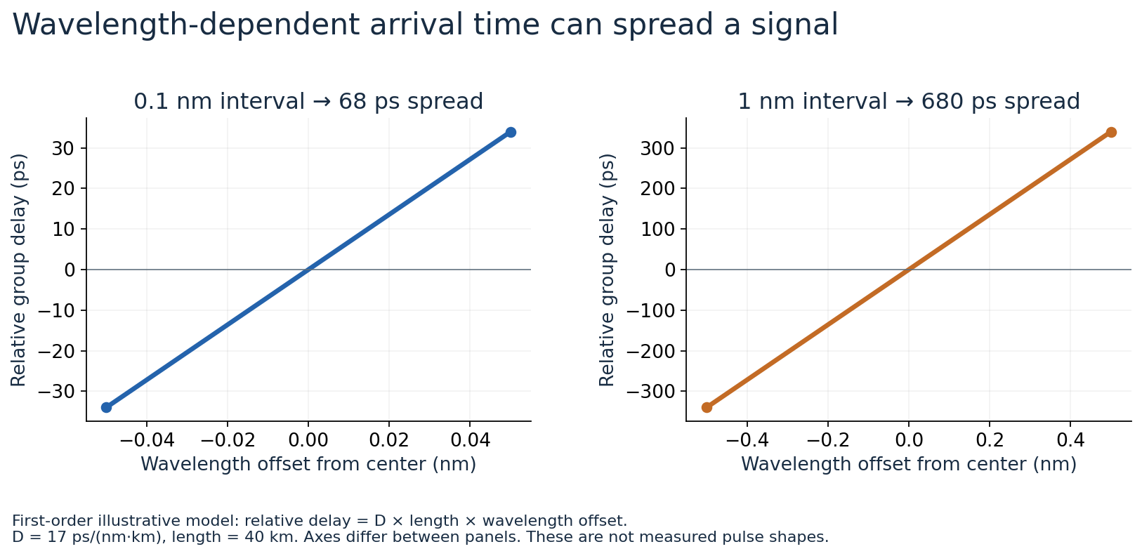
Figure 2. The linear model produces a 68 ps delay difference across a 0.1 nm wavelength interval and 680 ps across 1 nm. This plots differential group delay, not a measured pulse shape or a complete simulation of an optical transmitter and receiver.

Keep the same coefficient and length but increase spectral width to one nanometre. The corresponding delay spread becomes 680 picoseconds. This tenfold change follows directly from the linear approximation. It illustrates why the source belongs in a dispersion calculation, even when the cable has not changed. It does not establish that every transmitter with that nominal width will produce the same received eye diagram. Pulse shape, modulation, chirp, filtering, and receiver processing can change the full problem.

Compare the spread with the signaling timescale

For a deliberately simple binary signaling example at one gigabit per second, one bit interval lasts one nanosecond, or one thousand picoseconds. A sixty-eight-picosecond contribution is 6.8 percent of that interval. At ten gigabits per second, the interval is one hundred picoseconds, so the same contribution is sixty-eight percent. Nothing about the fibre calculation changed. The signaling timescale changed, making the same temporal spreading a much larger fraction of the interval available for distinguishing successive bits.

These fractions do not independently predict an error rate. There is no universal threshold at which a percentage in this calculation certifies every link as acceptable or failed. A real system's modulation, coding, receiver, equalization, and specified dispersion tolerance matter. The comparison is a screening calculation that identifies a potentially important constraint. It is useful precisely when we stop short of claiming more than it establishes and then consult the relevant system specifications or measurements.

Higher information rates also need not correspond to one binary decision per optical pulse. Multiple levels, polarization channels, and other arrangements alter the relationship between bit rate and symbol duration. I used binary signaling to make the arithmetic transparent. Applying the same one-over-bit-rate timescale indiscriminately to every optical format would be a mistake. The quantity to compare with a temporal impairment is the timescale of the actual waveform and receiver decisions, defined for the chosen system.

A power meter and a reflectometer answer different questions

A suitably configured source-and-power measurement can establish loss between defined endpoints. An optical time-domain reflectometer sends pulses and analyzes returned light to infer features along the fibre. EXFO's technical explanation describes the time-of-flight principle and the use of returned signals to locate events and characterize loss.[3] These are complementary views. One summarizes transmission across a boundary; the other can provide spatial clues about changes along the route.

In a simplified reflectometry calculation, distance is propagation speed multiplied by return time and divided by two, because the detected contribution traveled outward and back. Using an illustrative group index of 1.5 gives a propagation speed near two hundred million metres per second. A return after one hundred microseconds then corresponds to approximately ten kilometres. The group index is an assumption that must match the fibre and wavelength sufficiently well for the intended accuracy.

The instrument's trace is still an interpreted measurement. Strong reflections and finite pulse width can limit the ability to distinguish nearby events. Acquisition settings trade aspects of range, noise, and spatial detail. I would preserve those settings with the trace and avoid treating an automatically labeled event table as an infallible map. A localized feature can guide an investigation, but its interpretation needs the known route, connections, and measurement conditions.

A long quiet trace is not a dispersion certificate

An apparently satisfactory loss measurement or reflectometry trace does not, by itself, measure all relevant dispersion properties. The instruments and methods must match the quantity being claimed. If a high-speed link fails while the power budget appears sound, the next useful evidence may concern waveform quality, dispersion, configuration compatibility, or another impairment. Repeating the same loss measurement more precisely cannot establish a property that the measurement does not actually observe.

Consider two fictional fibres with the same measured endpoint loss but different group-delay behavior across the source spectrum. They can deliver the same average power and different temporal waveforms. Conversely, two paths can have similar temporal spreading but different attenuation. These comparisons show why separate columns in a specification are not redundant. Each constrains a different aspect of the received observation, and each can become the limiting factor under a different operating condition.

A change in wavelength can move both constraints at once. It may alter attenuation and chromatic dispersion, along with the compatibility of the transmitter, receiver, and other components. I would not generalize from one desirable change to an overall improvement without checking the other consequences. The phrase “this wavelength is better” needs a defined link, operating mode, and objective. A comparison that serves one system well can be irrelevant to another.

Investigate a rate-dependent failure without jumping to a cause

Suppose our fictional link works at a lower rate and fails at a higher one while average received power remains nearly unchanged. That observation is consistent with a timing-related limitation, but it does not prove dispersion. A mode mismatch, receiver behavior, configuration error, or another rate-dependent impairment could produce a similar symptom. The next step is to identify observations that differ between those explanations, using the equipment's documented capabilities and the known physical path.

I would establish the exact transmitter and receiver modes, their applicable limits, the fibre route, the operating wavelength, and the source's relevant characteristics. Then compare the measured loss and estimated dispersion with those limits. If a hypothesis predicts sensitivity to one controlled change, test that prediction where an authorized maintenance procedure allows it. A successful intervention is stronger evidence when the predicted intermediate measurement changes as well as the final error count.

Errors themselves need a denominator and context. Ten errors during a short interval and ten during a much longer interval do not describe the same behavior. Record the amount transmitted, the observation duration, the coding boundary, and whether the count is before or after correction. A receiver that corrects many errors can present a clean application stream while its physical margin changes. The reported metric should correspond to the claim about the layer being investigated.

Separate travel time from spreading in travel time

Our forty-kilometre fibre also has a propagation delay, even if every wavelength component arrived together perfectly. Using the same illustrative group index of 1.5, light travels at approximately two hundred million metres per second, so the one-way travel time is about two hundred microseconds. That common delay is a different quantity from the sixty-eight-picosecond differential delay calculated across the chosen spectral width. One describes when the signal arrives; the other describes how different components separate during the journey.

The scale difference is striking. Two hundred microseconds is two hundred million picoseconds. A relatively small variation around a large common travel time can matter when successive decisions are separated by only one hundred picoseconds. It would therefore be wrong to dismiss dispersion because it is tiny compared with the total journey time. The relevant comparison is with the temporal structure the receiver must distinguish, not simply with the duration of propagation from one endpoint to the other.

This also explains why a basic round-trip latency measurement is not a precise substitute for a dispersion measurement. It combines path delays and often processing or queueing, while the impairment of interest may concern differences across a narrow spectral interval. A test can be very accurate about the wrong quantity. Before commissioning a measurement, I would write the physical parameter required by the hypothesis and check whether the instrument actually estimates that parameter under the available conditions.

An uncertainty range is more useful than an unexplained margin

Return to the loss example and allow the assumed fibre coefficient to range from 0.24 to 0.27 decibels per kilometre. Across forty kilometres, the distributed contribution ranges from 9.6 to 10.8 decibels. Keeping the other modeled losses at 1.4 decibels gives total losses from eleven to 12.2 decibels. With the same zero-dBm launch, predicted received levels range from minus eleven to minus 12.2 dBm. This is a constructed bound, not a measured statistical confidence interval.

The worst end leaves 5.8 decibels above the assumed minus-eighteen-dBm sensitivity. After reserving three decibels, 2.8 remain. Showing the range explains how the coefficient uncertainty affects the conclusion. A single nominal value with a mysterious safety factor makes that relationship harder to inspect. Where uncertainties are correlated or specifications use different statistical meanings, they need an appropriate combination; simply adding convenient percentages can misrepresent the evidence.

We can perform the same kind of sensitivity check on the dispersion model. If source width increases from 0.1 to 0.2 nanometre while the other assumed quantities remain fixed, the calculated contribution rises from sixty-eight to 136 picoseconds. That identifies a variable worth measuring or bounding carefully in this particular model. It does not establish that replacing the source will cure a real incident. The value of the exercise is to rank which assumptions have enough influence to change the engineering conclusion.

Finally, preserve what changed between the nominal and conservative cases. Did we change a measured parameter, substitute a specification limit, or choose an allowance for future repairs? Those are different kinds of knowledge. Recording them separately makes it possible to update the budget when better evidence arrives. It also prevents the reserve from becoming a place where every unexplained discrepancy is hidden without anyone examining its cause or its likely range.

Keep the two budgets together

The useful engineering record contains both the power argument and the timing argument, with their assumptions visible. For our constructed link, the power calculation predicted minus 11.4 dBm, while the simple chromatic model predicted sixty-eight picoseconds across the chosen source width. Neither number is a complete verdict. Together they show which additional specifications and observations are needed to decide whether this particular communication system can recover its intended signal reliably.

This also changes how I would write an incident report. Instead of saying “the fibre is good” after one test, state which property passed which criterion at which wavelength and boundary. Instead of saying “dispersion caused the errors” after seeing a rate dependence, state the supporting measurement and competing explanations that were tested. Precision in the claim is more valuable than confidence in a broad label that the available evidence cannot justify.

The light can arrive weak, spread out, reflected, or altered in several ways at once. Communication depends on whether the receiver can recover the intended distinctions from that arrival. Attenuation and dispersion give us two different ways to examine the problem: how much optical power survives, and how propagation changes timing across the signal. Keeping both questions visible prevents a reassuring meter reading from becoming the end of an investigation that has only just begun.

References and method

1. Corning, Optical Fiber Glossary of Terms; attenuation, modes, and dispersion terminology.
2. Corning, Engineering Note 19: Dispersion; chromatic-dispersion mechanisms, units, and approximate spread calculations.
3. EXFO, The Fundamentals of an OTDR; returned-light measurements, event location, and instrument limitations.

Every numerical link and equipment limit is illustrative. The group-delay figure uses a constant dispersion coefficient over the plotted wavelength interval and does not simulate optical fields or predict bit-error rate. No installed fibre was tested for this article. Sources checked on 3 October 2026.

Explore the complete Signals Around Us series.