Seismic Waves as Evidence of Earthquakes

A line on a seismogram becomes restless, then suddenly much larger. It is tempting to read the image as a direct picture of an earthquake. But the instrument is at one location, while the source may be far away and deep underground. Between the source and the trace lie propagation through the Earth, the instrument's response, the timing system, and the processing used to display the record. The line is evidence from that chain. It is not a photograph of the fault.

This makes earthquake location an unusually clear example of inference from signals. We observe what arrived at several places and ask where and when an event could have produced those arrivals. The answer depends on both the observations and a model of how waves travel. A convincing result makes those two ingredients work together. It also reports how tightly the observations constrain the source, rather than treating the most precise-looking map marker as the most certain result.

The examples below use an intentionally simplified, uniform medium. Their wave speeds, source positions, and arrival times are constructed. They are not records from a real earthquake and must not be used as a regional travel-time model. The simplification lets us check every step of the arithmetic. We can then see why real location methods require more than a ruler and three circles on a flat map.

What the instrument has actually recorded

USGS describes seismograms as records of ground motion and cautions that not every wiggle is an earthquake: other ground vibrations and interference can appear in a record.[1] That distinction matters before any location calculation begins. A moving trace demonstrates variation in the recorded channel. Identifying its physical cause requires the waveform, timing, station context, and supporting observations. The largest visible excursion is not automatically the beginning of the event or the most informative feature for locating it.

Suppose a single station shows a short pulse while nearby stations show nothing comparable. Several explanations remain possible. The event may be local to that sensor, the other observations may be incomplete, or the signal may be too weak at their locations. The absence of matching traces does not select one explanation by itself. I would first check whether the comparison stations were operating and whether their records cover the relevant interval and frequency content. A network is useful only when the observations being compared are understood.

The vertical axis deserves equal attention. An enlarged display can make a small motion look dramatic. Two plots using different scales cannot be compared by the height of their wiggles alone. I would identify the channel, units, scale, and relevant instrument response before making a claim about relative motion. The horizontal axis needs its time reference and sample spacing. These details are not decoration around the signal. They determine what comparisons the signal can support.

Different arrivals provide a clock for distance

USGS distinguishes primary, or P, waves from secondary, or S, waves. P-wave motion involves compression and expansion along propagation; S-wave motion is transverse. P waves generally arrive before S waves along the relevant paths because they travel faster.[2] Their differing arrival times provide information about the journey. The useful observation is not simply that the trace became large. It is identifying particular arrivals that can be compared with predictions from a propagation model.

Choose a uniform model with P-wave speed 6 kilometres per second and S-wave speed 3.5 kilometres per second. Let both travel a straight distance D from the same source to one station. The travel times are D/6 and D/3.5 seconds. Their difference is D × (1/3.5 − 1/6). In this invented medium, that becomes approximately 0.11905 seconds per kilometre. A larger separation between these identified arrivals corresponds to a longer path.

If the S arrival follows the P arrival by twelve seconds, our model gives D = 12/0.11905, or 100.8 kilometres. We did not need the source's origin time for this calculation because subtracting the two arrival times cancels it. That cancellation is useful, but it does not cancel errors in identifying the phases or in the assumed speeds. The result is only as appropriate as the quantities and model used to derive it.

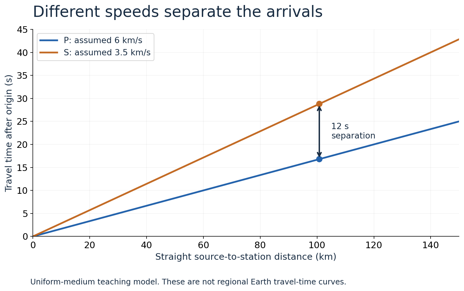
Figure 1. Uniform-medium calculation, not an Earth travel-time table. At 100.8 km, the model predicts P and S travel times of 16.8 and 28.8 seconds, separated by 12 seconds.

The two speeds here are teaching assumptions, not universal constants for the Earth. USGS's explanation of earthquake location explicitly requires a velocity model under the seismic network to calculate predicted travel times.[3] A real path can pass through materials with different properties. Applying our one-line calculation to an arbitrary record would hide that structure. The simple model helps explain the role of arrival differences; it does not replace the model needed for a particular region, depth, and set of phases.

There is another subtlety in the distance. D is a source-to-station path length in our straight-ray model. If the source is below the surface, that is not automatically the horizontal distance to the epicenter. The hypocenter is the source location at depth; the epicenter lies above it at the surface. A map can display the latter while the travel-time calculation constrains the former. Mixing those definitions can create a geometrical error before any uncertainty in wave speed is considered.

For a numerical illustration, suppose the straight source-to-station distance is 50 kilometres and the source depth is 30 kilometres in a flat, uniform model. The horizontal separation is the square root of 50 squared minus 30 squared, which is 40 kilometres. Drawing a 50-kilometre surface circle would therefore use the wrong radius for that stipulated depth. The difference is not a flaw in the arrival-time measurement. It is a consequence of converting a three-dimensional distance into a two-dimensional picture.

Why one station cannot supply the whole location

With only the P–S difference in our isotropic model, every point at the same source-to-station distance gives the same result. We have learned a distance constraint, not a direction. To make the geometry visible, temporarily reduce the problem to an entirely two-dimensional plane with source and stations all in that plane. This is an illustrative construction. It allows circles to represent the distance constraints without pretending that depth has been determined from a real surface network.

Place station A at coordinates (0, 0), station B at (120, 0), and station C at (0, 100), all in kilometres. Put the constructed source at (45, 40). Its distances from A, B, and C are approximately 60.21, 85, and 75 kilometres. In our chosen velocity model, the corresponding S-minus-P intervals are approximately 7.168, 10.119, and 8.929 seconds. Those are calculated observations whose generating source we know because we chose it.

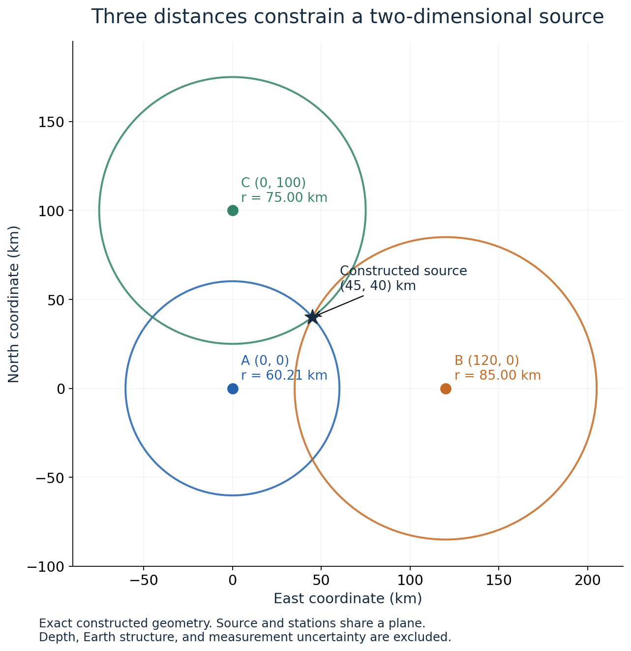
Figure 2. Exact distances in a flat two-dimensional demonstration. The source and stations are stipulated to share the plane. Real earthquake location includes depth, travel-time modeling, and observation uncertainty.

A single circle leaves many possible positions. Two circles generally leave two intersections when the geometry permits them. A third independent distance can distinguish those alternatives in this exact two-dimensional construction. USGS uses the meeting of distance constraints to introduce location from multiple stations.[4] The diagram's value is to show why additional observations constrain the answer. Its limit is that real arrival times rarely produce perfectly intersecting circles, and real sources are not restricted to our drawing plane.

Change the source while keeping its distance from A fixed and A's P–S interval remains unchanged. Stations B and C may see different intervals. That gives us a way to understand the information added by the network: it tests candidate locations that one station cannot distinguish. More stations are not simply repetitions of the first observation. Their different positions can add different geometrical constraints, provided their arrivals and timing are trustworthy and the propagation model connects them consistently.

Network geometry matters. In an extreme invented arrangement, put every station along the same straight line and consider two source positions mirrored across that line in the same plane. Their distances to every station are identical. No number of perfectly measured distances from stations on that line separates the mirror images. A station off the line breaks this symmetry. This example shows why the placement of observations can matter as much as their count when an inverse problem has an ambiguity.

The origin time is another unknown

Arrival time combines the time the source began with the time the wave took to travel. If a P wave reaches a station at 12:00:20 and the model predicts a ten-second journey, the inferred origin time is 12:00:10. But a different candidate source position may imply a different travel time. Location and origin time must be made consistent across the network. Subtracting P and S arrivals was one way to eliminate origin time in our simple calculation; it did not determine the origin time itself.

For our constructed station A, the P travel time is approximately 10.035 seconds. Choose an origin time of 100 seconds on an arbitrary common clock. The P arrival is then about 110.035 seconds, while the S arrival is about 117.203. Their difference remains 7.168 seconds. Shift the origin time by five seconds and both arrivals shift by five, but their difference stays the same. This separates information about the event's timing from information contained in the travel-time difference.

USGS describes an iterative location approach: choose a trial location, depth, and origin time, predict arrivals, compare them with observations, and adjust the trial to improve the fit.[3] The differences between observed and predicted times are residuals. Their pattern contains information about the adequacy of the candidate explanation. A fit is a relationship between data and a model, not a declaration that the model has become the Earth. Unmodeled structure or problematic picks can still affect the inferred source.

To see what a residual means, imagine our trial predicts an arrival at 110.0 seconds and the observed arrival is 110.3. The residual is positive 0.3 seconds under the convention observed minus predicted. Perhaps the source is farther away than the trial suggests; perhaps the assumed speed is too high; perhaps the picked arrival is late. One residual alone cannot separate those explanations. Comparing residuals across stations and phases is more informative than treating every mismatch as a location adjustment.

Suppose every arrival is delayed by almost the same amount relative to the trial. Changing the origin time is an obvious hypothesis to test. Suppose the mismatches vary systematically with station direction or path. That suggests examining other parts of the model as well. These are diagnostic ideas illustrated by our equations, not a claim that one residual pattern uniquely proves one cause in field data. A good analysis tests whether the proposed adjustment improves the relevant observations without creating new inconsistencies elsewhere.

Picking an arrival is itself a measurement

In the clean diagram, the arrivals have exact labels. In a recorded waveform, identifying the onset can be less straightforward. A gradual emergence above background variation does not announce one unambiguous sample as its beginning. Different choices can produce different travel times. I would want the original waveform, the selected phase label, and an estimate of picking uncertainty available for review. A table of arrival times can look exact even when some entries represent substantially less certain judgments than others.

Our simple formula quantifies the consequence. Since D equals 8.4 times the P–S interval in this model, an interval error of 0.1 seconds changes the inferred distance by 0.84 kilometres. An error of one second changes it by 8.4 kilometres. These numbers follow from the chosen speeds, not from a universal seismological conversion. They are useful because they make the timing uncertainty visible in the same units as the map. A tiny-looking timestamp difference can have a meaningful spatial consequence.

Clock errors require a careful distinction. A constant offset in one station's clock cancels when subtracting that station's P and S times, assuming both use the same offset. It does not cancel when comparing its absolute arrivals with those at another station. A clock rate error or a timing discontinuity between the two arrivals can also affect their difference. The helpful cancellation in one calculation is therefore not permission to ignore timing integrity throughout the network.

I would also ask whether the selected arrivals belong to the same event. Imagine two sources occur close enough in time that their records overlap. Pairing one event's P arrival with another event's S arrival could produce a plausible-looking interval and a meaningless distance. The calculation cannot detect that mistake simply because it returns a positive number. Event association belongs before inversion. Observations need to be grouped through consistent timing and waveform evidence, not merely proximity in a list of detected peaks.

A good fit can still depend on a wrong assumption

Return to the twelve-second interval, but change the stipulated speeds to 6.2 and 3.6 kilometres per second. The conversion becomes D = 12/(1/3.6 − 1/6.2), approximately 103.02 kilometres. The same interval now yields a distance about 2.22 kilometres larger than the earlier 100.8. We have not altered the recorded time. We have altered the propagation model used to interpret it. This is a concrete reason to distinguish observational uncertainty from uncertainty in the model.

It is possible to report many decimal places for either result. Those digits would describe arithmetic precision, not establish the correctness of the speeds. I would round a public explanation to match its evidence and preserve the model information alongside the more detailed internal result. A map coordinate without an uncertainty description can suggest that the source is known more tightly than the observations support. A useful estimate tells the reader both where the best-fitting source lies and how that conclusion depends on the available evidence.

An independent station can challenge the interpretation. Fit a candidate using some observations, then compare its predictions with another suitable record. A successful prediction adds information beyond reproducing the data used to obtain the fit. A mismatch is worth examining rather than automatically discarding the new record. The station may reveal a poor pick, a timing issue, or a limitation in the propagation model. The comparison is useful because it creates an opportunity for the explanation to fail.

Removing difficult observations can make almost any fit look cleaner. Sometimes a record should be excluded because it is demonstrably unsuitable, but the reason should be documented. I would distinguish a known timing failure from an inconvenient residual whose cause is still uncertain. The retained and excluded observations together help another analyst assess the result. A small residual after unexplained exclusions is weaker evidence than a transparent fit that acknowledges where its model does not yet explain the record.

Location, size, and local shaking are separate claims

An estimated source location answers where the event originated under the model. It does not by itself establish its magnitude or the shaking experienced at every community. USGS distinguishes an earthquake's magnitude from intensity, which varies with location.[4] That separation matters when a seismogram is shared publicly. A dramatic trace at one station is evidence about that observation. Converting it into a statement about the event's size or local effects requires the appropriate analysis and additional context.

Consider two fictional recordings displayed at different gains. The first fills the screen while the second appears modest. Without scale information, their visual heights cannot rank the underlying motions. Even with comparable units, station location and propagation conditions still matter for interpreting the source. The right response is to identify what has been normalized or corrected before comparing amplitudes. A striking image can introduce a question, but it should not quietly supply a measurement the caption never defined.

The time order also limits the claim. These calculations interpret waves that have already been generated and observed. They are not predictions of when a future earthquake will begin. Conflating detection, location, and prediction gives a signal more authority than the method provides. This article explains how observations constrain an event after its signals arrive. It does not offer a warning algorithm or a method for forecasting a particular future event.

Before trusting a plotted point, I would also ask how its uncertainty is drawn. In our two-dimensional circle example, an uncertain distance is better imagined as a band than an infinitely thin circumference. Several bands can overlap over an area rather than at one exact point. The geometry of that overlap matters: it may be narrow in one direction and broad in another. Reporting one rounded distance around the estimate can hide that directional difference.

A useful follow-up observation targets the weak constraint. If two candidate positions predict almost identical arrivals at the existing stations but different arrivals elsewhere, a suitable additional record can distinguish them. The choice follows the model's predictions, not merely a preference for more data. This is the same logic that made the off-line station useful in our mirror-image example. Observation placement is part of how uncertainty is reduced.

What the final explanation should preserve

A useful account of our constructed source would state the station coordinates, the selected P and S arrivals, the assumed speeds, and the two-dimensional restriction. It would show that the source at (45, 40) reproduces the calculated distances and intervals. It would then explicitly stop short of claiming that three surface stations always determine a unique real hypocenter. The explanation becomes stronger by making its exact achievement inspectable rather than extending it beyond the model we actually solved.

For a real network result, I would look for corresponding information about stations, phases, timing quality, the velocity model, residuals, and location uncertainty. These elements let a reader distinguish a newly computed estimate from a fully resolved description of the source. Later observations or model improvements can revise an estimate without invalidating the idea of measurement. The revision should be traceable to changed evidence or assumptions. Science becomes harder to trust when that reasoning is hidden behind an unexplained replacement of one precise number with another.

The important signal is not one wiggle in isolation. It is the agreement, and sometimes the disagreement, among observations that a common source should explain. P and S arrivals, station geometry, and a propagation model turn recorded motion into constraints on an event we cannot directly watch underground. Keeping those constraints visible is what makes the inference useful. The seismogram starts the investigation; the network and the model tell us how far the resulting explanation can reasonably go.

References and method

1. USGS, About the Seismograms; reading displayed records and recognizing non-earthquake contributions.
2. USGS, Seismographs: Keeping Track of Earthquakes; P and S waves and arrival-time constraints.
3. USGS, How Do Seismologists Locate an Earthquake?; velocity models, trial hypocenters, origin time, and residual fitting.
4. USGS, The Science of Earthquakes; wave motion, introductory location geometry, magnitude, and intensity.

The figures and numerical examples are original calculations in explicitly simplified models. No actual event, regional velocity profile, operational location result, or forecast is represented. Sources checked on 3 October 2026.

Explore the complete Signals Around Us series.