Sonar and the Time of a Returning Echo

A short pulse leaves a sensor and disappears into the water. A fraction of a second later, something returns. On a screen it becomes a line, a bright patch, perhaps a reassuring number labelled depth. The sequence feels direct: send sound, hear the echo, measure what is below. But the number has crossed several interpretive steps. The instrument observed a returning signal. Converting that observation into a distance, a position, and an explanation of the reflecting surface requires more information.

That is what makes sonar a useful subject for this series. The basic arithmetic is approachable, while the difference between a demonstration and a dependable survey is substantial. We can calculate a range in one line and still be wrong about the water depth or the identity of the object. Rather than hide that complexity, I want to follow it from the simplest echo to the questions a convincing interpretation would have to answer.

NOAA distinguishes active sonar, which emits sound and receives returning echoes, from passive sonar, which listens without sending its own probing pulse.[1] This article concentrates on a constructed active-sonar example. None of the diagrams shows an actual survey, wreck, fish school, or deployment. The timings and geometry are invented so that every calculation can be inspected. The published references explain the physical and surveying context; the worked numbers are ours.

The factor of two has a physical meaning

Assume a stationary transducer sends a pulse toward a stationary reflector through water with a uniform sound speed of 1,500 metres per second. The echo returns 0.4 seconds after transmission. Multiplying speed by time gives 600 metres. But that is the total outward-and-return path length. Under our straight, symmetric path assumption, the one-way range is half of it: 300 metres. The factor of two accounts for a journey, not a mathematical convention added to make the answer convenient.

We can write this simple model as range = sound speed × round-trip time / 2. Each term needs a definition. The time begins at the acoustic transmission event used by the system and ends at the identified return. Any uncorrected delay in the instrument's timing chain can enter the result. The speed must describe propagation along the path well enough for the intended accuracy. The range is measured from the acoustic reference point, which is not automatically the water surface or the vessel's navigation antenna.

In the same model, a one-millisecond timing difference corresponds to 0.75 metres of range. A ten-millisecond difference corresponds to 7.5 metres. These numbers give a useful scale for an investigation. If a displayed range shifts by several metres, I would ask whether the identified arrival moved, whether a different return was selected, or whether another conversion parameter changed. Calling the shift “sensor noise” skips the opportunity to compare the symptom with the quantities that actually determine the result.

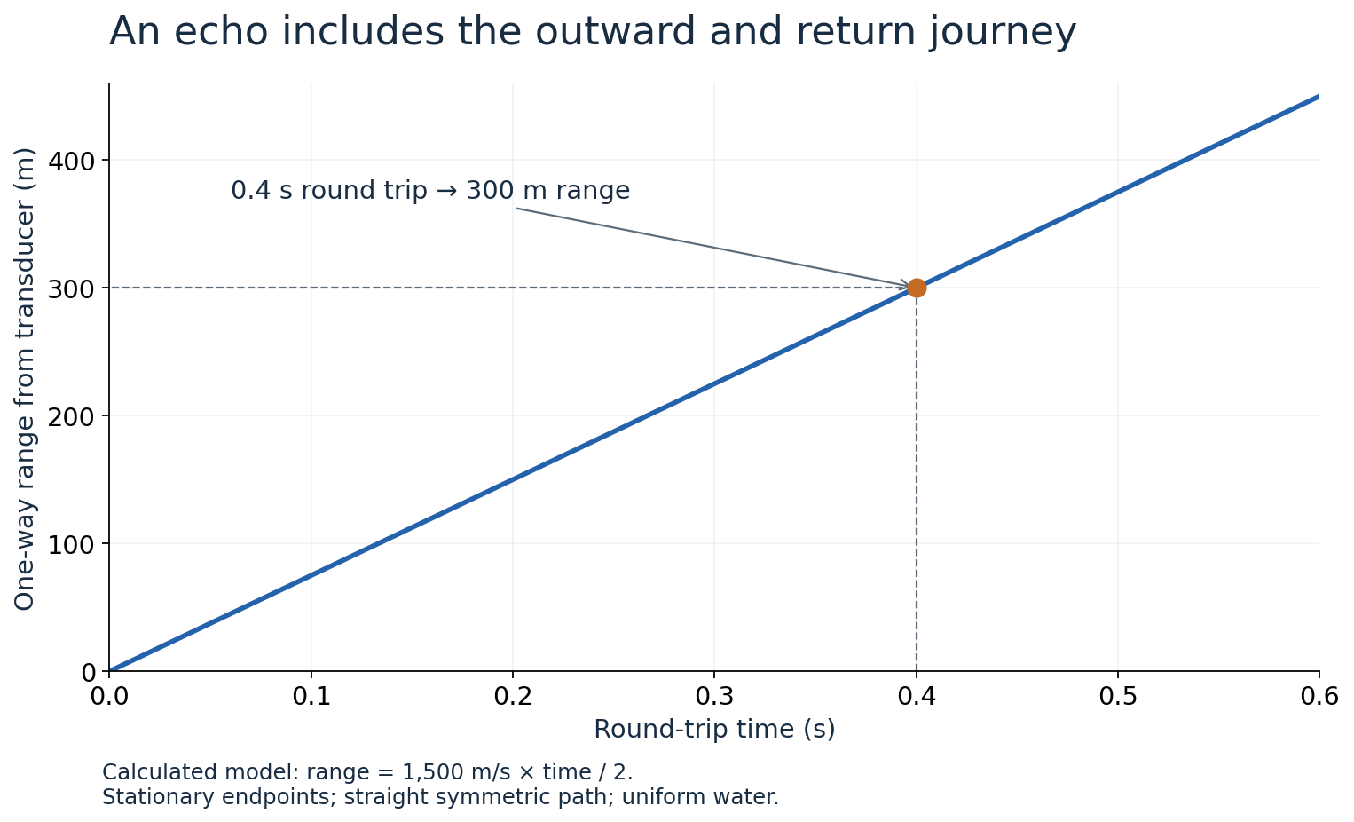
Figure 1. A straight, symmetric outward-and-return path with stationary endpoints. The assumed speed is 1,500 m/s. The graph gives range from the transducer, not automatically charted depth.

The transmitted pulse also occupies time. Imagine an idealized rectangular pulse lasting one millisecond and two otherwise identical point reflectors at slightly different ranges. Their returned pulse envelopes begin at different times. If the range separation is 0.3 metres, the start times differ by 0.4 milliseconds in our model, so the envelopes overlap. This constructed example shows why recording timestamps finely is not the whole resolution problem. The transmitted waveform, received shape, and processing determine what separate echoes can be distinguished.

It would be misleading to turn that simple example into a universal sonar-resolution formula. Systems can use different waveforms and processing methods, and a real reflector may be extended rather than point-like. Our calculation establishes only the overlap of two specified pulse envelopes. It nevertheless supplies a useful question for reading a specification: does the quoted number describe timing increments, separation of two targets, uncertainty in one target's range, or spacing between displayed pixels? Those are different claims.

The water is part of the measuring system

Now keep the observed round-trip time at 0.4 seconds but change the actual uniform sound speed in our fictional scene to 1,460 metres per second. The correct one-way range becomes 292 metres. Software that continues using 1,500 reports 300 metres, an eight-metre overestimate. The echo timing has not become less precise. The conversion from time to distance is using the wrong scale. This is the acoustic version of a measuring ruler whose markings do not match its assumed length.

Discovery of Sound in the Sea, an educational resource from the University of Rhode Island and the Inner Space Center, explains that seawater sound speed depends on temperature, salinity, and pressure.[2] Those properties can vary with position and depth. Consequently, one convenient nominal speed is not a complete description of every survey path. In a real project, I would want to know what sound-speed information was acquired, where and when it was acquired, and how the processing used it.

The eight-metre difference in our example is not a claim about the usual error of any instrument. It follows from deliberately chosen speeds. The same arithmetic lets us assess another assumed mismatch: a one-percent error in the speed produces a one-percent range error when the measured time is fixed in this model. At a nominal range of 300 metres, that is about three metres. Such calculations help determine which input deserves better measurement before additional digits are added to the display.

If speed changes along the path, the travel time reflects those different segments. For an illustrative straight path consisting of 100 metres at 1,500 metres per second and 100 metres at 1,450, the one-way time is 100/1500 + 100/1450 seconds, approximately 0.13563 seconds. The round trip is about 0.27126 seconds if it retraces the same path. Multiplying that by 1,500 and dividing by two reports approximately 203.45 metres, although the stipulated one-way distance is 200 metres.

This segment calculation assumes the path is already known. In the ocean, changes in sound speed can also refract sound and alter its route, as the DOSITS sound-channel tutorial explains.[3] A curved route adds a geometric problem to the speed problem. I would therefore avoid correcting a complex survey by replacing one scalar value and assuming every beam is repaired. The appropriate propagation model and measured water conditions belong together. Our straight-path examples isolate the arithmetic so that this added requirement remains visible.

A range is not necessarily a depth

Return to the 300-metre one-way range. Suppose the straight beam points 30 degrees away from vertical. The vertical separation is 300 × cos(30 degrees), approximately 259.8 metres. The horizontal separation is 300 × sin(30 degrees), or 150 metres. Reporting the full 300 metres as vertical depth would add about 40.2 metres in this invented geometry. Nothing is wrong with the round-trip timing; the error comes from assigning a slanted distance to the wrong axis.

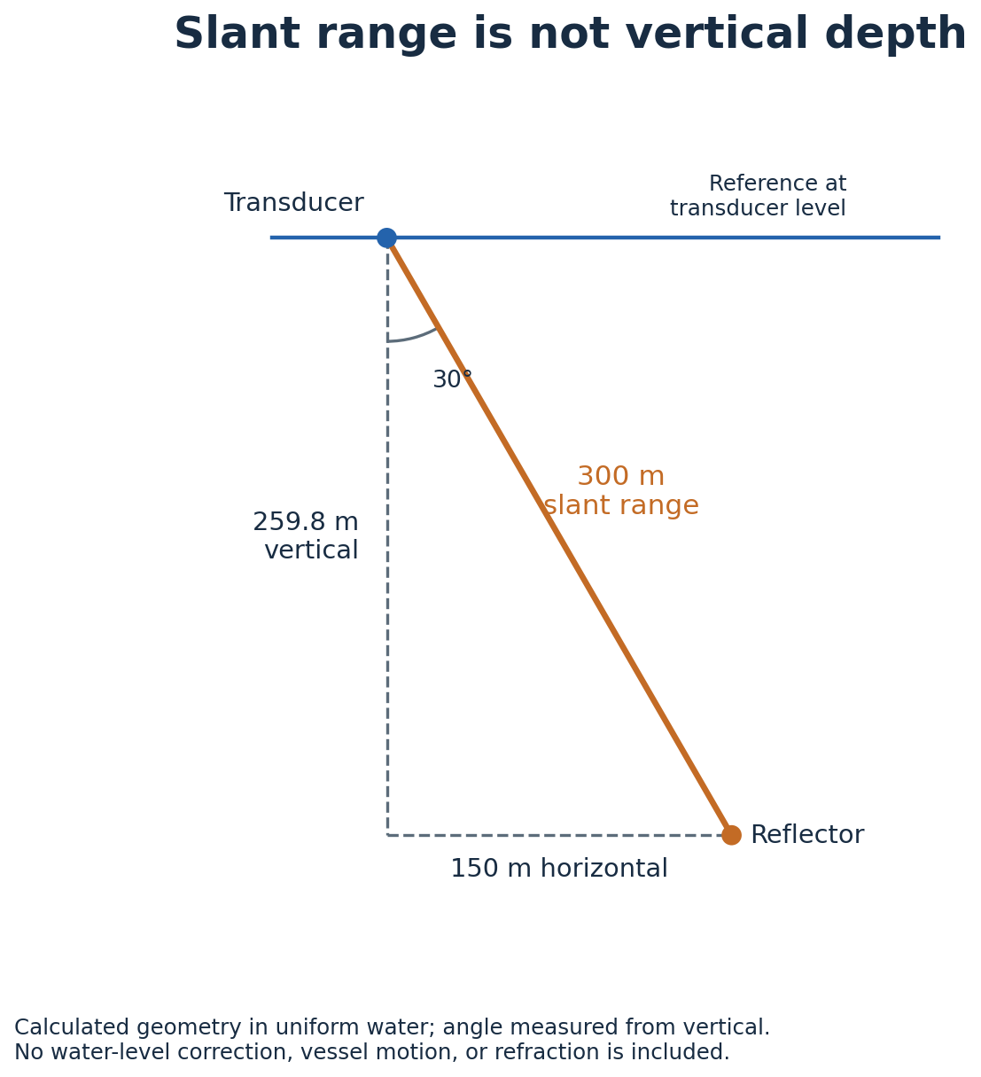
Figure 2. Calculated straight-ray geometry in uniform water. Angles are measured from vertical. Vertical separation is relative to the transducer; this sketch does not include vessel motion, water-level corrections, or ray bending.

Now imagine the transducer is two metres below the chosen water-surface reference. Under the additional assumption of a flat, stationary surface, the reflecting point lies about 261.8 metres below that surface. The range from the transducer, vertical separation from the transducer, and depth below the surface are three different quantities. A further reference may be used for a nautical chart. Before comparing two depth numbers, I would establish their reference surfaces and corrections rather than assume they describe the same distance.

NOAA's account of a 2015 survey in Kotzebue Sound explicitly identifies measuring sound speed through the water column and recording and correcting vessel motion as parts of multibeam surveying.[4] That is a useful concrete reminder that the sonar is one part of a measurement system. The platform's orientation and position affect where a return is placed. A sharply timed echo cannot compensate for an unknown pointing direction when the aim is to locate a feature on a map.

We can estimate the importance of an angle in our fictional scene. Keep the slant range at 300 metres. At 29 degrees from vertical, the vertical component is approximately 262.4 metres; at 31 degrees it is approximately 257.2. A one-degree change around our chosen angle changes that component by roughly 2.6 metres. This calculation does not define a survey tolerance. It shows why an orientation measurement can matter even when the range measurement appears stable.

The location of the observation in time matters for the same reason. A moving vessel occupies different positions when the pulse leaves and when the echo arrives. A real processing system must account for the relevant geometry and timing conventions. Our diagram freezes the platform to keep the calculation elementary. I would make that simplification explicit in a teaching illustration and remove it before interpreting a moving-platform dataset. Otherwise the clean diagram silently becomes a claim about a system it did not model.

The first bright return may not be the bottom

Suppose our fictional record contains a return at 0.18 seconds and another at 0.40 seconds. Using the original 1,500-metre-per-second assumption gives ranges of 135 and 300 metres. The timings establish two candidate path lengths under the model. They do not, on their own, label the nearer return a fish or the farther return the seabed. We need information about beam direction, surrounding returns, signal strength, and the scene before choosing those interpretations.

NOAA's split-beam sonar description explains that echoes can arise from contrasts in density or sound speed within the surrounding water and describes observations of both the water column and seafloor.[5] This broadens the possible scene beyond a single hard bottom. A sonar record can contain information from multiple structures along the beam. An instrument or analyst choosing a bottom return therefore makes a classification decision as well as a timing measurement. The decision rule needs evaluation against the intended environment.

In an invented classification rule, let the software select the strongest return within a time window. If the 0.18-second return becomes stronger than the 0.40-second one, the displayed range jumps from 300 to 135 metres even though both reflecting features remain stationary. The jump is caused by a change in selection, not necessarily movement of the bottom. Retaining the underlying echo record would let an investigator distinguish those possibilities. Saving only the selected depth removes much of the evidence needed to explain the change.

An alternative rule might select the first return above a threshold. That creates a different sensitivity: a weak early reflection becoming just strong enough to cross the threshold can move the selected range abruptly. The threshold may be necessary, but it is part of the observation process. I would want its value, any automatic gain adjustments, and the confidence or quality flags preserved with the result. A single range number can conceal several decisions made before it reaches the user.

This is also why a missing return should be handled as missing evidence rather than automatically converted into “nothing is there.” The transmitted pulse may not illuminate the intended feature, the received signal may fall below the relevant detection rule, or the observation may be incomplete. Those are possibilities to investigate, not explanations chosen in advance. A system that can report detection limits and acquisition state gives its users a more useful absence than a blank region whose meaning is unspecified.

Strength and distance answer different questions

NOAA distinguishes bathymetry, derived from echo travel time, from backscatter, which measures returning sound strength.[6] Backscatter can help characterize the seafloor when interpreted with other information. The two measurements are related through the same acoustic observation but are not interchangeable. A bright region in a return-strength image is not automatically a tall object, and a deep point need not be weak simply because its display uses a dark color. The image legend must tell us what the colors represent.

Imagine two maps of the same invented area. One assigns brighter colors to shallower depth. The other assigns brighter colors to stronger returns. A bright patch could coincide in both maps, appear in only one, or have different boundaries. Without the legend, a reader might tell a persuasive story about a ridge from an intensity pattern alone. I would show the measurement quantity and units prominently, then explain any inference about material or shape separately from the underlying mapped value.

The acquisition settings also belong in a comparison of brightness. Suppose the received signal is multiplied by a larger gain before display while the physical scene remains unchanged. Its plotted strength increases even though the reflector did not become harder or larger. Our simplified example needs no detailed acoustic model to establish that possibility. A before-and-after claim about the seabed should therefore account for calibration and processing settings, rather than compare screenshots whose color scales may have changed.

There is a familiar temptation to turn a striking sonar image into an immediate identification. A shape resembles a wreck, a line resembles a pipe, or a cluster resembles fish. Resemblance can guide the next observation, but a defensible identification needs additional evidence suited to the claim. The sound has registered a response from a scene through a particular geometry and processing chain. Calling that response a named object is another step. I want the explanation to show where that step became justified.

Which transmitted pulse produced the return?

The time calculation also needs the correct starting event. Imagine a simplified instrument transmitting indistinguishable pulses every 0.25 seconds while a distant reflector produces a 0.40-second round trip. The first pulse's echo arrives 0.15 seconds after the second transmission. If an elementary detector incorrectly associates that echo with the most recent pulse, it calculates 112.5 metres using our 1,500-metre-per-second assumption instead of the stipulated 300 metres. The arithmetic is consistent; the event association is wrong.

This invented ambiguity is not a claim that a modern sonar necessarily makes that mistake. It explains why the transmitted sequence and the permitted range window belong in the interpretation. A system may distinguish transmissions through its waveform design or other processing. An investigator must establish which method is actually used before assigning an arrival to a particular outgoing pulse. A precise timestamp cannot rescue a calculation whose start and finish describe different journeys.

The reporting lesson is practical. Preserve enough information to reproduce the pairing between a transmission and its selected return. If a range changes when the transmission interval changes, that relationship can suggest a testable explanation. It should be compared with the predicted timing, not treated as proof by itself. Changing an instrument mode may change several settings together, so the entire relevant configuration should accompany the comparison.

How I would test a suspicious depth jump

Begin with the original records around the jump rather than the final map alone. Did the selected arrival time change? Did the processing switch between two persistent echoes? Did the assumed speed or beam angle change? Did a quality flag appear? These questions separate mechanisms that could produce a similar displayed symptom. Their order should follow what the system actually records. An investigation becomes inefficient when it demands a measurement the instrument never saved while ignoring a more direct observation that is available.

Next compare adjacent observations and, where possible, an independent pass under documented conditions. A stationary feature should occupy a consistent location after the relevant transformations, within their uncertainties. If the apparent jump follows a processing setting rather than a geographical feature, that suggests a different explanation. Repeated passes are not automatically independent evidence: they can repeat the same calibration error. The useful comparison changes or checks a suspected cause while keeping other conditions sufficiently understood.

I would write predictions before adjusting a setting. If selecting the nearer echo caused the jump, reprocessing the retained record with a justified alternative selection should change which arrival supplies the result. If the error arose from the assumed sound speed, the correction should follow the time-to-range scaling or the appropriate ray model. A prediction ties the proposed cause to an observable consequence. Without it, almost any improvement after a change can be described as confirmation, even when the reason remains unknown.

For a small teaching experiment, known stationary targets and an explicitly simplified environment can provide a reference. Compare the predicted return times with observed ones, then change one distance or angle. In a real survey, the reference methods and uncertainty requirements are more demanding. The underlying discipline is the same: the reference must test the quantity being claimed. Measuring a target's slant distance does not independently validate a water-level correction or a geographical coordinate transformation.

The final record should separate acquired observations from processed products. Transmission timing, received waveform or relevant echo features, navigation, orientation, sound-speed information, and processing choices contribute different pieces. A finished map can be easier to use, but keeping the relationship back to those pieces makes corrections and reviews possible. Otherwise a later reader sees only the attractive endpoint of a chain and cannot tell which assumption would need to change if the result is challenged.

The echo is a question the water answered

Active sonar is powerful because it controls part of the experiment. We know when a probing signal was sent and can look for a related return. That makes range estimation possible under a propagation model. It does not make the ocean a uniform ruler or turn every reflection into an identified object. Passive listening begins with different information because the observer has not supplied the same known transmission event. The method should match the available evidence rather than borrow the certainty of another arrangement.

The simple 0.4-second echo took us through a surprisingly long chain: round-trip time, assumed sound speed, one-way range, beam geometry, vertical reference, return selection, and interpretation of the scene. Each step can be tested and documented. Skipping one may still produce a clean number, which is why the number alone is a poor guide to the quality of the investigation. The useful question is what information supports each conversion between the received sound and the statement printed on the map.

When I look at a sonar display, I want to know what the instrument actually heard before deciding what the picture means. That does not make the picture less valuable. It connects its value to a method another person can inspect. A returning echo is evidence of an acoustic path and a response along it. A dependable depth or identification comes from explaining how that evidence was turned into the claim, including the assumptions the water itself did not label for us.

References and method

1. NOAA National Ocean Service, What Is Sonar?; active and passive observation.
2. University of Rhode Island and Inner Space Center, Discovery of Sound in the Sea, Tutorial: Speed of Sound; dependence on seawater properties.
3. Discovery of Sound in the Sea, Tutorial: Sound Channel; refraction in a varying sound-speed field.
4. NOAA Office of Coast Survey, Report from the Arctic: Surveying Kotzebue Sound 2015; sound-speed and vessel-motion observations in a survey.
5. NOAA Ocean Exploration, Split-Beam Sonar; acoustic returns from the water column and seafloor.
6. NOAA National Ocean Service, How Does Backscatter Help Us Understand the Sea Floor?; travel-time and return-strength products.

All numerical scenes and figures are constructed. Straight-path calculations assume stationary endpoints and the stated uniform speeds unless segmented propagation is explicitly specified. They are explanations of measurement principles, not navigation products. Sources checked on 3 October 2026.

Explore the complete Signals Around Us series.