A Connected Call with Silence at Both Ends

The phone says the call is connected. The timer advances. Both people say hello, wait, and say hello again. Nothing comes back. From the user's perspective this is one failure: the conversation does not work. Inside the system, however, several different operations may have succeeded. Treating the entire call as one indivisible event makes troubleshooting frustrating because evidence about one operation gets mistaken for evidence about all the others.

I would begin with a narrower question: what exactly does “connected” describe in this application? A successful session exchange can coexist with an unusable audio path. SIP provides mechanisms for establishing, modifying, and terminating sessions; it is not the speech itself.[1] The screen may be accurately reporting the state the application reached. The mistake is extending that report into a claim that microphone capture, media transport, decoding, and sound output all worked.

This investigation uses a deliberately constructed call between endpoint A and endpoint B. It is not a report of an outage on my infrastructure or anybody else's. The addresses, counters, and timings are examples chosen so readers can follow the reasoning. We will keep the two directions separate, identify what each observation establishes, and work toward a diagnosis only when the evidence distinguishes it from alternatives. The aim is to make the investigation reproducible, not to turn one memorable symptom into a universal fix.

Draw the media path before reading the counters

Suppose a signaling service helps A and B establish the session, while the negotiated media is intended to travel directly between the endpoints. That is one possible arrangement. Another system may place a media relay or a telephony server between them. The actual arrangement matters because a capture at a signaling server may contain no speech packets by design. An empty capture at a node outside the media route is not evidence that the sender failed to produce audio.

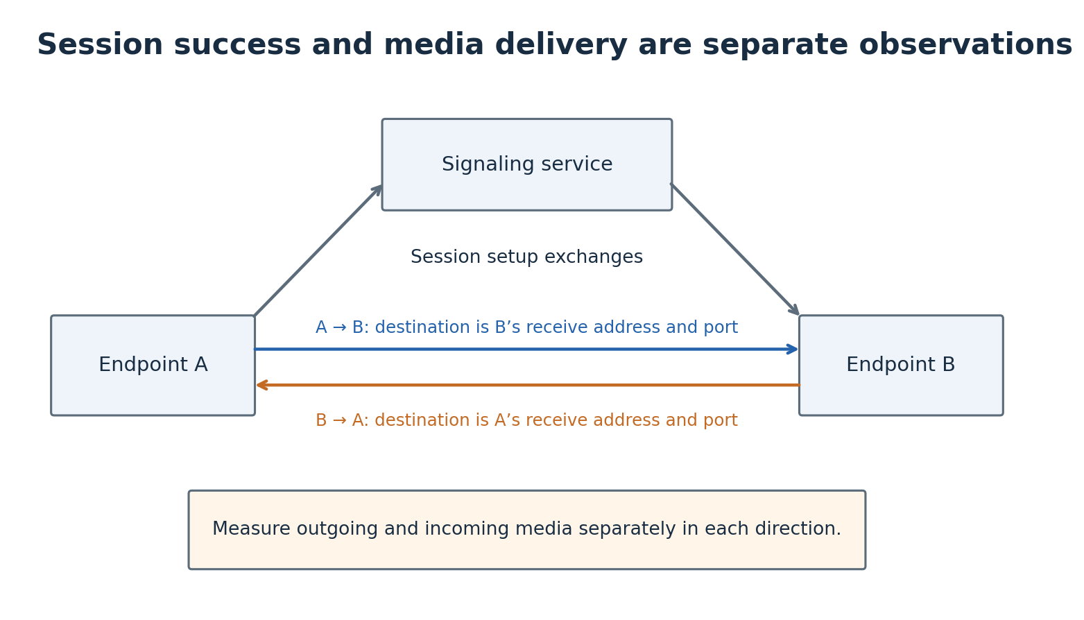
Figure 1. The fictional investigation assumes direct media between A and B. Signaling passes through a separate service. Real deployments may anchor media at a relay or server; the capture locations must follow the actual route.

I would write down where A's outgoing media should go and where B's outgoing media should go. Then I would identify the points where those expectations can be checked. These are two flows with separate source and destination details, not a single bidirectional object that either exists or does not. One-way audio is possible, and a report of silence at both ends should be tested in both directions. A combined packet total can conceal a complete failure of one flow.

The capture plan should name the call interval, the interface or observation point, and the identifiers used to associate records with this call. A busy telephony service can carry many simultaneous streams. Seeing some RTP traffic proves little unless it belongs to the relevant participants and time. Likewise, a signaling dialog identifier and a media-source identifier serve different purposes. I would record how the application or negotiated session maps the two rather than assume every number in adjacent logs refers to the same conversation.

Read the agreement as an agreement

The offer-and-answer model in RFC 3264 describes how participants negotiate media streams and their receiving addresses, ports, formats, and directions.[2] In a send-and-receive unicast exchange, the offer tells the peer where the offerer wants to receive; the answer provides the corresponding information for the answerer. That description establishes intended behavior. It does not independently prove that packets can reach the advertised destinations from the other side of the network.

For our example, suppose A intends to receive audio on UDP port 40000 and B on port 42000. A should send its outgoing stream to B's receiving destination, while B sends to A's. This is easy to reverse when reading a large trace quickly. I would label each extracted value with its owner and role: “A's advertised receive port,” for example. A table with those labels is more useful than a loose list of addresses copied out of a signaling log.

SDP, specified in RFC 8866, supplies the session description syntax, including media descriptions and mappings between RTP payload types and encodings.[3] A fragment such as m=audio 42000 RTP/AVP 0 describes an audio media entry with a port, profile, and payload format. It is only a fragment, not a complete session description. Connection information, relevant attributes, and any media-level overrides must be interpreted together. Copying one line out of context can preserve the syntax while losing the destination the peer actually uses.

I would also inspect the negotiated direction. A stream marked inactive does not promise two-way speech. Send-only and receive-only descriptions need to be interpreted from the participant that supplied them, and a later exchange may change the session.[2] This creates an important time dimension: the first description in a call log may no longer describe the media when silence occurs. Hold, resume, transfer, or another session update can create a new interval with different expectations.

For the constructed case, we stipulate that the current agreement is two-way audio using a common format. That eliminates one branch of the investigation by assumption. In a real call, it would need evidence from the actual exchange and application state. I would keep both the original and updated descriptions in the incident record, with their times. Otherwise a packet capture can be judged against an obsolete destination and appear wrong even when it follows the latest agreement.

A ten-second interval with no arrivals

Now collect observations over a fictional ten-second interval after setup. A emits 500 media packets toward B's advertised destination. B emits 500 toward A's. At the corresponding receiving boundaries, neither expected stream is observed. We assume the capture methods are functioning and cover the relevant interfaces and interval. Those qualifications are part of the evidence: without them, “zero received” could describe an incomplete observation rather than a failed delivery.

The first result is narrower than “the microphones are broken.” Both endpoints generated packets. That does not prove those packets contain speech, but it tells us there is an outgoing media process to investigate. The absence at the receiving boundaries puts attention on the destinations and the intervening path. I would compare the actual destination addresses and ports in the outgoing packets with the negotiated receiving values, then ask whether those values are reachable from the other endpoint's network.

Imagine the addresses advertised in the constructed exchange belong to internal networks with no route between them. The signaling service remains reachable, so setup can complete, but sending media toward those internal destinations does not produce the intended delivery. This explains how the connected indicator and silence can coexist. It is still a hypothesis until the routing and packet evidence support it. A private-looking address alone is not proof of a defect: private networks can be deliberately interconnected.

Asterisk's PJSIP NAT documentation provides a concrete implementation example of why signaling and media addressing need separate attention.[4] It discusses local network definitions, external media and signaling addresses, and whether media stays through Asterisk. Those options illustrate roles in a particular configuration model. They are not interchangeable switches to enable blindly. A setting that keeps media on a server changes the intended route, so the observation points and the network permissions must match that new route.

For our hypothetical case, a controlled correction supplies receiving destinations that are actually reachable in the intended topology. A repeat call then shows the expected streams arriving at both boundaries. That result supports the addressing explanation, especially if the remaining conditions are held constant. But the investigation has not yet proved audible speech. We have moved from “no observed delivery” to “observed arrival.” The next boundary is whether the application accepts and decodes the arriving media.

Packets can arrive without becoming sound

RTP provides sequence numbers, timestamps, payload-type identification, and source identification, among other transport functions.[5] These fields help organize the stream, but the existence of an RTP-shaped packet does not demonstrate successful playback. A receiver can reject an unsupported payload type or encounter a mismatch with the negotiated format. The investigation should compare the arriving stream with the current session description and the receiver's processing records, not stop at the first packet visible in a network capture.

Suppose the receiver reports 500 arrivals but zero decoded audio frames. That is a different boundary from the earlier example. Routing toward the observed interface now has evidence in its favor, while acceptance, format interpretation, security processing, or another receive-stage issue remains to be examined. These are candidate explanations, not conclusions from a counter alone. The useful next observation is the receiver's reason for accepting or rejecting those packets, with the same stream and time interval identified.

Suppose instead that the receiver produces decoded samples and its output meter moves, but the listener still hears nothing. Attention shifts again. Which output device is selected? Does the application send audio to that device? Is the expected channel being monitored? These questions can be tested with a known local sound and application-level observations. A working network path does not establish the final acoustic result, just as a moving microphone meter does not establish successful delivery to the other person.

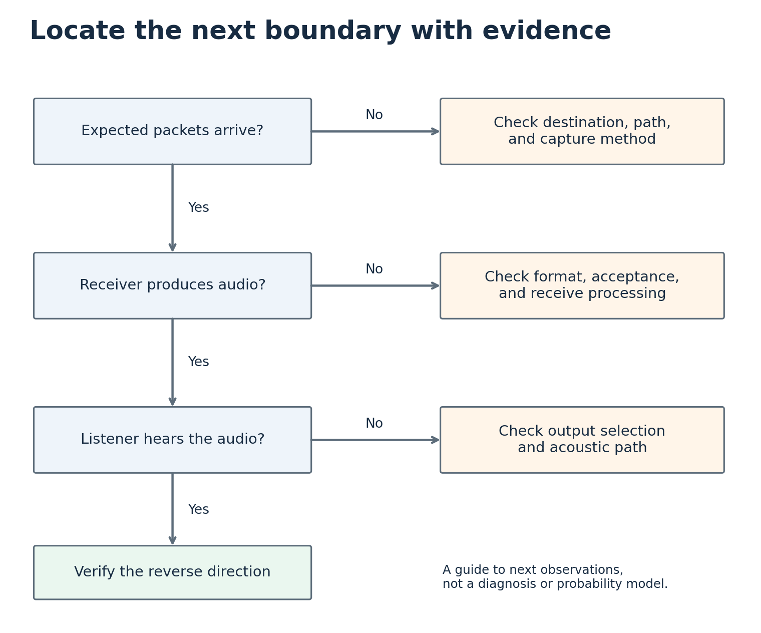
Figure 2. Each observation selects a next investigation boundary. The diagram does not assign probabilities or identify a universal cause. Check the observation method before interpreting an absent counter or capture.

I would use a controlled test source to distinguish content from transport when appropriate. For example, a known tone injected at a documented point can test the path after that point. If injected after microphone capture, however, its successful arrival does not validate the microphone. The injection location belongs in the report. Otherwise a useful partial test gets retold as an end-to-end success. Every shortcut in the test path excludes some component from the evidence it can provide.

Count what this codec should produce

Our 500-packet example assumes a continuous stream with one packet every 20 milliseconds. That gives 50 packets per second, or 500 in ten seconds. Choose mono PCMU for the worked calculation: the RTP audio/video profile assigns it an 8,000-hertz clock and eight-bit samples.[6] Twenty milliseconds therefore contain 160 samples, which occupy 160 payload bytes. Different formats, packetization intervals, silence behavior, or session changes require different expectations. The calculation should follow the actual negotiated and observed stream.

For this simple example, add a 12-byte basic RTP header, an 8-byte UDP header, and a 20-byte IPv4 header without options. The resulting IP packet is 200 bytes. At 50 packets per second, that is 80,000 bits per second in one direction. Two such directions total 160,000 bits per second. This arithmetic excludes link-layer overhead, tunneling, security additions, control traffic, and any extra headers. It is a scoped packet-budget example, not a universal bandwidth estimate for a phone call.

The distinction between payload rate and carried traffic matters when comparing counters. Someone might expect 64 kilobits per second from the encoded audio and see 80 kilobits per second at an IP accounting point. In our constructed case, both values are correct for their respective boundaries. Before calling the difference waste or unexplained traffic, identify what the counter includes. A useful measurement names the layer and interval. “The call uses 80” is not enough: eighty what, where, and over which period?

The sequence and timestamp fields add another consistency check. In our continuous 20-millisecond PCMU example, consecutive packets advance the sequence number by one and the media timestamp by 160, ignoring wraparound for this short illustration.[5] Initial values need not start at zero. A gap between observed sequence numbers raises a question about missing observations or missing delivery; it does not identify where the packet disappeared. Comparing evidence at multiple boundaries is what turns that gap into a localized finding.

Consider seeing sequence numbers 1000, 1001, 1003, and then 1002 at a capture point. The fourth arrival changes the interpretation of the apparent gap after the third. If a reporting tool immediately treats the gap as permanent loss, its summary may need revision. For a live receiver, arrival order and usefulness for playback can also differ. The packet might eventually appear in a saved capture while arriving too late for the intended listening schedule. A complete investigation distinguishes eventual arrival from timely use.

Time changes the diagnosis

To make that distinction concrete, imagine an intentionally simple playback rule: each packet must arrive within 60 milliseconds of its corresponding generation time. Four fictional packets are generated 20 milliseconds apart and experience delays of 35, 40, 95, and 45 milliseconds. All four eventually arrive, but the third misses our stipulated deadline by 35 milliseconds. The capture can honestly report complete eventual arrival while the application cannot use every packet at its planned playback time. This is an illustrative rule, not a specification for a real jitter buffer.

Now increase that invented deadline to 100 milliseconds. All four packets fit, but the receiver has accepted a longer wait before playback. The calculation exposes the trade: tolerating more delay variation can increase conversational delay. It does not establish an optimal setting for an actual deployment. That would require its arrival patterns, application behavior, codec handling, and user requirements. I would avoid changing a buffer simply because a single graph has spikes without first identifying what those spikes measure.

Clock interpretation matters too. Comparing timestamps from two hosts requires an account of their synchronization and timestamp locations. If one record marks packet generation and another marks application processing after a queue, the difference includes more than network travel. A tidy subtraction can still compare unlike events. For the fictional timing example, we stipulated a common clock and precisely defined events. A real report should state how it achieved an equivalent basis or acknowledge the uncertainty in its delay estimates.

The same discipline applies to summaries. An average over an entire call can hide a brief interval of silence. I would align the user's reported symptom with a smaller time window and compare before, during, and after it. If silence begins immediately after a session update, that temporal relationship suggests a specific place to inspect. It is not proof that the update caused the failure, but it offers a more discriminating next step than repeatedly restarting everything involved in the call.

Connectivity checks provide another kind of evidence

Some systems use ICE to gather possible network paths and evaluate candidate pairs. RFC 8445 defines that framework, including connectivity checks and selection procedures.[7] Such checks add information beyond merely announcing a receiving address. They do not replace the rest of the audio investigation. A usable network path still needs the agreed media processing and working input and output. Nor should an investigator assume every SIP deployment uses ICE; the actual session and implementation determine which mechanisms exist.

For a system that does use it, I would preserve the selected candidate pair and any later changes alongside the failure interval. The address first displayed in an initial description may not be the path ultimately selected. If a relay is involved, observations should follow both sides of that relay. The general principle remains the same: draw the actual route supported by current evidence, then place measurements on that route. A diagram copied from a generic tutorial is only a starting hypothesis.

Make the repeat test capable of failing

A repeat test should challenge the correction rather than merely look for a green indicator. In our addressing example, I would ask A to send a known spoken phrase while B confirms what was heard, then reverse the direction. The phrases should be different so that a local echo or mistaken monitor cannot easily stand in for the remote path. The application counters and negotiated destinations would be recorded during that same interval. This combines the human outcome with evidence about the path that produced it.

If A hears B but B still cannot hear A, the overall label should remain one-way audio. It would be misleading to declare the call repaired because the total received packet count became nonzero. The successful direction is useful evidence, but the unresolved direction needs its own observations. I would compare the two flows to find the earliest boundary where their evidence differs. That comparison can be more efficient than repeating every check on both sides without using what already works.

The observation method needs its own control. If a capture reports no media on an interface where a known working comparison call produces packets, that comparison strengthens confidence in the setup, provided the intended routes are equivalent. If both calls appear empty, I would first question the capture location or filtering. A failed observation instrument can imitate the symptom under investigation. Demonstrating that it detects a relevant positive example is a practical way to narrow that possibility.

Finally, I would preserve the exact change made between attempts. If the team simultaneously changes codec selection, media routing, endpoint software, and firewall policy, a successful call establishes that the new combination works but identifies no single cause. Sometimes restoring service requires several changes quickly; the report can say that honestly. Where conditions allow, a controlled change with a predicted result produces a more useful explanation. The distinction matters later when someone tries to apply the supposed fix to a different failure.

What a useful incident record would say

The report for our constructed addressing failure should state that session setup completed, both endpoints emitted media toward the advertised destinations, and the corresponding arrivals were absent at validated observation points. It should explain the routing mismatch found, identify the controlled correction, and record the repeat-call results. If decoded audio and audible output were also checked, say so separately. That creates a chain from symptom to observation to correction to verification instead of compressing everything into “NAT issue fixed.”

I would also record what the test did not establish. A successful repeat call over one path does not prove every remote network, codec, transfer, or hold-and-resume case behaves identically. This is a boundary on the conclusion, not a reason to withhold a demonstrated fix. It helps decide which follow-up checks matter. If the correction specifically changes media routing, testing the relevant call transitions is more informative than repeating unrelated registration checks that already passed.

The people on the call do not need a lecture on protocol layers when they ask why they cannot hear. They need the conversation restored. But restoring it reliably depends on keeping those layers distinct during the investigation. The timer, the negotiated description, the packet counter, the decoded samples, and the audible output each report something different. When we ask each observation only what it can answer, the silence becomes a set of testable boundaries rather than one large, frustrating mystery.

References and method

1. IETF, RFC 3261: SIP — Session Initiation Protocol; session control roles.
2. IETF, RFC 3264: An Offer/Answer Model with SDP, especially unicast streams and direction attributes.
3. IETF, RFC 8866: SDP — Session Description Protocol; media description syntax and payload mappings.
4. Asterisk, Configuring res_pjsip to Work Through NAT; implementation-specific addressing and media-path example.
5. IETF, RFC 3550: RTP — A Transport Protocol for Real-Time Applications, especially the fixed header and reception reporting.
6. IETF, RFC 3551: RTP Profile for Audio and Video Conferences with Minimal Control; PCMU format and static payload assignment.
7. IETF, RFC 8445: Interactive Connectivity Establishment; candidate gathering, checking, and selection.
8. IETF, RFC 768: User Datagram Protocol and RFC 791: Internet Protocol; header sizes used in the packet-budget calculation.

The call, packet counts, addresses implied by the scenarios, and playback deadlines are constructed examples. No private traffic or real incident is represented. The packet-budget example assumes standard 8-byte UDP and 20-byte IPv4 headers without options. Sources checked on 3 October 2026.

Explore the complete Signals Around Us series.