One Message Arriving Along Several Paths

A radio link works at one position and struggles a short distance away. The transmitter is unchanged, the receiver is still nearby, and the battery is not the explanation. It is easy to imagine radio coverage as a smooth pool of signal that becomes gradually weaker with distance. A real environment can be more complicated. The receiver may encounter several versions of the same transmitted waveform, arriving along different routes and combining differently at each position.

That combination is the subject of this investigation. A reflection does not arrive with a label saying which wall it encountered. The antenna responds to the resulting electromagnetic field, and the receiver has to recover information from that result. Depending on their relative amplitudes, phases, and delays, contributions from different paths can reinforce or reduce one another. A short movement can therefore change reception without a comparable change in the overall distance between the devices.

Cisco's technical explanation of multipath describes signals reaching a destination both directly and after reflections, with their combination affecting reception.[1] The examples below reduce that complex environment to two idealized paths. Their numbers are constructed, not measurements from a room or a particular wireless product. The model will let us calculate a fade, examine its frequency dependence, and identify what additional observations would be needed before diagnosing a real link.

The receiver adds waveforms, not explanations

Begin with two sinusoidal contributions at the same frequency. Let the first have normalized amplitude one. Let the second also have amplitude one and arrive in phase. Their sum has amplitude two. Now shift the second by half a cycle while leaving the amplitudes equal. At every instant it is the negative of the first, and their sum is zero. This complete cancellation is an ideal limiting case. It requires the specified amplitudes, phase relationship, and observation point.

The message did not become less important when the waves opposed one another. The transmitter did not decide to stop halfway through the explanation. The change occurs in the physical combination arriving at the receiver. That is why describing the situation only as “the signal got weaker” leaves an important mechanism hidden. The weakness may be the result of individually substantial contributions adding to a small total, rather than every contribution becoming small independently.

Equal contributions are not necessary for a deep variation. Set the second amplitude to 0.7 while keeping the first at one. With zero phase difference, the combined amplitude is 1.7. With a half-cycle difference, it is 0.3. The corresponding squared amplitudes are 2.89 and 0.09 in normalized power-like units for the same impedance. The ratio is about 32.1 to one, or approximately 15.1 decibels. A large change appears even though the two individual amplitudes were held fixed throughout the calculation.

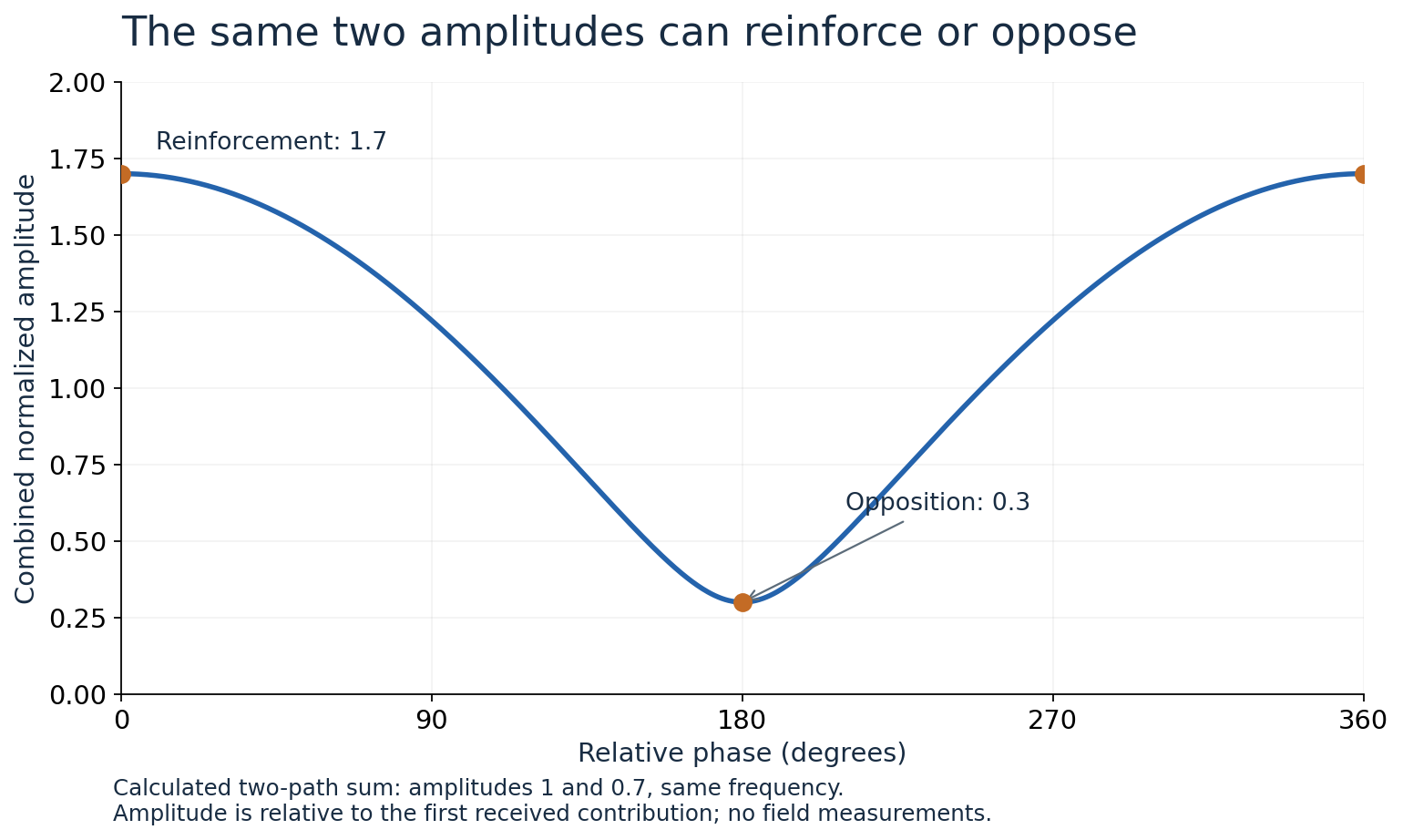
Figure 1. Calculated magnitude of 1 + 0.7 exp(jφ). The two path amplitudes are fixed; only their relative phase changes. Units are normalized to the first received contribution, not to transmitted power.

At intermediate phase differences, we cannot simply add or subtract the amplitude numbers. They represent oscillations whose peaks occur at different times. The squared magnitude of the sum is 1 + 0.7 squared + 2 × 0.7 × cos(φ), where φ is the relative phase. Taking its square root gives the curve in the figure. This equation makes the mechanism auditable: the cross term changes with phase while the two individual squared amplitudes remain constant.

The example does not create energy when the amplitude rises or destroy it universally when the local sum falls. We are describing a field combination at a particular receiver location and with a particular coupling to its antenna. A complete physical energy accounting includes the spatial field and the environment. Our normalized two-component calculation is not a transmitter power budget. Keeping that distinction explicit prevents a local constructive-interference result from being retold as an amplifier that generated extra energy without a source.

A small path change can be a large phase change

For a sinusoid, a propagation path longer by one wavelength adds a full cycle of phase delay. A half-wavelength difference adds half a cycle, before accounting for any additional phase change associated with reflection and the rest of the path. Using approximately 300 million metres per second for propagation, a 2.4-gigahertz wave has a wavelength of about 0.125 metres. Half of that is 6.25 centimetres. The exact vacuum speed of light underlying this approximation is defined in SI.[3]

That does not mean moving every receiver by 6.25 centimetres always switches a good link into a bad one. The relevant quantity is the change in the difference between path lengths, together with the paths' other amplitude and phase changes. A movement can lengthen one route and shorten another, affect both similarly, or change which reflections are important. The geometry determines the relationship. The wavelength calculation gives a scale for phase sensitivity; it does not supply a universal placement rule.

For a constructed case, assume one path length stays fixed while the other increases by 6.25 centimetres at our approximate wavelength. If their relative phase initially produced reinforcement and all other factors remain fixed, that extra distance changes the relative phase by half a cycle. The pair moves toward opposition. In a different geometry where both paths lengthen equally, their phase difference remains unchanged even though their absolute travel times increase. Relative delay is what controls this particular interference pattern.

Reflection itself also belongs in the model. It can alter the contribution's amplitude and phase, so distance alone is not sufficient to label a real reflection constructive or destructive. I would avoid drawing two geometric routes, subtracting their lengths, and announcing a precise null without describing the relevant reflection and antenna behavior. The simple phase calculation is most useful when its assumptions are stated. Otherwise a neat wavelength argument can conceal missing physical information.

One signal can experience different channels across frequency

Now describe the two paths by a relative delay rather than a chosen phase. Let one received contribution be our reference and let the other arrive 50 nanoseconds later with amplitude 0.7. At a propagation speed of approximately 300 million metres per second, that delay corresponds to 15 metres of additional path length. We also choose the relative phase to be zero at a reference frequency. These assumptions define a mathematical channel whose frequency response we can calculate.

Changing the frequency by an amount Δf changes the relative phase by 2π × Δf × 50 nanoseconds. An offset of 10 megahertz gives half a cycle, moving the two contributions from reinforcement to opposition in this model. An offset of 20 megahertz gives a full cycle and restores the original relative phase. The combined power response therefore repeats every 20 megahertz. No receiver motion is needed for this variation across frequency; it follows from the fixed delay difference.

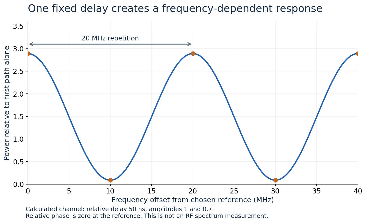
Figure 2. Squared magnitude of 1 + 0.7 exp(−j2πΔfτ), with τ = 50 ns and zero relative phase at Δf = 0. Power is normalized to the first path alone. This is a constructed channel response, not a spectrum measured in a room.

Robert Gallager's MIT material models wireless channels as combinations of delayed contributions and discusses the relationship between delay spread and variation across frequency.[2] That framework explains why a single signal-strength value may miss an important part of the problem. A wide signal can occupy frequencies where the channel response differs substantially. Averaging their energy into one number can hide which portions were suppressed and what distortion the receiver must handle to recover the data.

Our plot provides a concrete comparison. A narrow probe near the chosen reference sees a strong sum, while one near the 10-megahertz offset sees a much weaker sum. A signal spanning both regions experiences a response that is not a single constant multiplier. The word “strong” is therefore incomplete unless it names the measurement bandwidth and frequency. The same physical two-path arrangement can look favorable to one narrow measurement and problematic to another.

There is a useful inversion here, but it has limits. If a measured channel response shows regularly spaced ripples, a delayed contribution is one hypothesis to examine. In our exact two-path model, a 20-megahertz repetition corresponds to 50 nanoseconds. A real response may contain more paths, instrument effects, or frequency-dependent components, so the observed ripple does not automatically identify a particular reflecting wall. The calculation suggests a candidate delay that further evidence can test.

Delayed copies can reach later symbols

So far we have used sinusoids to expose phase. A message-bearing waveform changes with time. In a simple baseband model, write the received signal as the current transmitted waveform plus 0.7 times a delayed copy, with the relevant phase included in the path coefficient when necessary. If the delay is significant compared with the waveform's changes, part of an earlier symbol can overlap a later one. The channel then has memory: the present received value depends on more than the present transmitted symbol.

Consider a discrete teaching example in which the echo arrives exactly one symbol interval later and has a real coefficient of 0.7. The received sample is y[n] = x[n] + 0.7x[n−1]. Let symbols take values plus one or minus one. If the current and previous symbols are both plus one, the received value is 1.7. If the current is plus one and the previous is minus one, it is 0.3. The same current symbol produces different observations because the preceding symbol contributes too.

Now let the current symbol be minus one. With a preceding plus one, the received value is −0.3; with a preceding minus one, it is −1.7. In this noiseless example, a zero threshold still separates the signs, but the weaker observations sit much closer to the decision boundary. Add a constructed disturbance of magnitude 0.4 with an unfavorable sign and those weaker cases can cross it. This illustrates why considering only the strongest received amplitude gives a poor account of decision robustness.

The example does not claim that a real modem samples an unprocessed waveform with this elementary rule. Receivers can estimate and compensate for aspects of the channel, and actual modulation may use more complex symbol sets and processing. The point is to identify the problem that processing addresses. A delayed contribution changes the relationship between transmitted and observed symbols. Evaluating the receiver means testing how well it handles that relationship under the relevant noise and channel conditions.

We can even write a noiseless correction for our stipulated model if the previous symbol is known: subtract 0.7 times that previous symbol from the received sample. The result is the current symbol. But if the previous decision was wrong, this correction can introduce another error. Likewise, an incorrect echo coefficient leaves a residual. The small example makes clear that compensation depends on information about the channel and the sequence. It is not a magical operation that removes every echo without consequences.

A stationary link can still have a changing environment

Neither device has to move for a path contribution to change. A reflecting or obstructing part of the environment can change position or condition. Gallager's discussion includes time-varying paths and the resulting channel model.[2] For an investigation, the important observation is how the received response changes with time and which environmental or configuration changes coincide with it. A stationary transmitter-receiver separation does not establish a stationary propagation environment.

Imagine a fictional link whose reception changes when a large movable panel is repositioned. That is a clue, but it does not by itself prove a particular reflection model. The panel could alter more than one route or block a contribution. I would compare repeated measurements at documented panel positions while keeping the devices and settings fixed. If the effect repeats, we gain evidence connecting the configuration with reception. To identify the detailed mechanism, we would need measurements that distinguish the remaining path explanations.

Time averaging can conceal this behavior. Suppose received power alternates between the high and low values in our two-path calculation during different intervals. One average does not reveal how long the weak intervals last or whether they coincide with failed transmissions. A data application may tolerate some interruptions differently from a live voice application. The evaluation should preserve the timing of the received conditions and the application's failures rather than assume the average predicts the experience.

This also changes how I interpret a successful test. A link that transfers a file once at a fixed position has demonstrated that transfer under those conditions. It has not established performance throughout every likely environmental state. A useful test plan follows the intended use: relevant positions, orientations, motion, and time variation. The aim is not to make an infinite checklist. It is to test the conditions that the proposed explanation says can materially change the link.

Separate propagation from other possible failures

A failed radio link does not automatically establish multipath. Interference from another source, receiver limitations, configuration changes, and failures elsewhere in the network can produce overlapping symptoms. I would first define what failed: detection of a waveform, decoding of frames, successful delivery, or the application task. Evidence about one boundary should guide the next observation. Repeatedly changing antenna placement while the actual failure is beyond the radio would produce activity without addressing the cause.

For a constructed experiment, suppose a local receiver reports changing decoded-frame errors while a separate wired portion remains stable. That gives us a reason to examine the radio path. We would then compare those errors with frequency, position, and channel measurements if available. If only an internet application is slow and no radio observations have been collected, the inference is much weaker. A symptom at the end of a chain needs intermediate evidence before it can be assigned to one physical mechanism.

The measuring instrument can also influence the apparent channel. Cables, connectors, antennas, calibration, and receiver settings contribute to what is recorded. A ripple observed in a measurement setup may originate in the setup rather than the room. A useful control changes or characterizes the measurement path while preserving the channel question. I would want calibration and configuration records attached to the response plot, especially before interpreting a feature as a specific physical reflector.

Diversity needs different evidence paths

Cisco's discussion uses antenna diversity to illustrate obtaining reception from different antenna observations in a multipath environment.[1] The broad idea is to avoid depending entirely on one unfavorable realization of the channel. The implementation depends on the radio: selecting one observation, combining observations, and transmitting separate streams are different operations. An older product's switching description should not be treated as a universal description of every multi-antenna system.

An elementary example shows what diversity can and cannot promise. Suppose receiver observation A has a deep reduction at one location while observation B has a stronger usable signal at that same moment. A system able to use B may avoid the immediate failure. If both observations are affected identically, merely possessing two readings adds less protection. The useful resource is a relevant difference between the observations and processing that can use it, not the antenna count printed on a product box.

Nor is blindly adding two receiver voltages always beneficial. Our opening calculation already showed how two substantial contributions can cancel when their phases oppose. Combining observations coherently requires accounting for their relationship. A diagram that shows two antennas converging into one box should therefore explain what that box does before promising an improvement. Selection, estimation, and combining rules are part of the system being evaluated. The physical branches alone do not guarantee the desired result.

A channel estimate also needs a timestamp. In our symbol example, suppose the receiver assumes an echo coefficient of 0.7 while the actual coefficient has changed to 0.5. Subtracting the estimated echo leaves an error of minus 0.2 times the previous symbol. The correction now changes sign according to the sequence. A previously successful estimate has become a source of structured residual error. Measuring the channel once is useful only for as long as its relevant behavior remains sufficiently similar.

This creates a practical balance between observation and use. Updating the estimate more often consumes measurement opportunities and processing effort, while updating too slowly can leave the receiver using stale information. The appropriate interval depends on the channel's changes and the application's requirements. Our calculation does not select that interval, but it identifies what a test should examine: how performance changes as the gap between channel estimation and data reception grows.

Test the explanation before choosing the remedy

For the imaginary room, I would start by recording a repeatable baseline: fixed device positions, orientations, frequency settings, transmitted test pattern, and the relevant receive and delivery measurements. Then change one condition that the multipath hypothesis predicts will matter. A small position change or a controlled reflector change may produce a discriminating result. The test should record both successes and failures, because selecting only the favorable new position can hide how sensitive the improvement remains.

A frequency comparison can be similarly useful if the equipment and authorization permit the intended test. Our two-path model predicts a specific response across frequency. A real measurement that follows a comparable pattern supports investigating delayed contributions, but it must be separated from changes in antenna response, noise, or interference. The goal is a controlled comparison, not an assumption that changing the channel and seeing improvement proves the original problem was multipath.

I would reserve a separate observation for checking the proposed remedy under conditions not used to choose it. If repositioning was selected after examining several points, a later test across the intended operating conditions provides more useful evidence than repeating the best point alone. A remedy can be appropriate without validating every detail of the original hypothesis. The report should distinguish “this configuration improves the measured outcome” from “this specific reflecting surface has been conclusively identified as the cause.”

The final explanation should retain the model's scale and limits. Our 0.7-amplitude echo produced a fifteen-decibel range between constructive and destructive combinations. Our 50-nanosecond delay produced a twenty-megahertz response repetition. Those relationships are exact within the stated models, but their numerical values were chosen. A real installation needs its own measurements before inheriting them. The examples supply questions and calculations that make an investigation sharper; they do not diagnose an unseen room.

One message arriving along several paths is a reminder that more arriving energy does not translate automatically into an easier decoding problem. The receiver encounters a combined waveform with structure in time, frequency, and space. Understanding that structure helps explain why a small move can matter, why a single strength number can mislead, and why a well-designed receiver needs more than a louder input. The useful investigation follows the paths through their observable consequences instead of treating the radio environment as a smooth, invisible wire.

References and method

1. Cisco, Multipath and Diversity; reflected-path combination and an implementation-specific diversity example. Product-specific advice in this older document is not generalized here to modern radios.
2. Robert Gallager, MIT OpenCourseWare, Chapter 9: Wireless Digital Communication, 2006; delayed-path models, time variation, and channel measurement.
3. NIST, SI Units: Length; the metre and the defined vacuum speed of light.

All amplitudes, delays, geometries, and symbol examples are constructed. Figures use analytic two-path models with stated normalization and fixed coefficients. No field survey, equipment benchmark, or universal antenna-placement rule is represented. Sources checked on 3 October 2026.

Explore the complete Signals Around Us series.