ADC Resolution Is Not Measurement Accuracy

A sensor display changes from 1.65 volts to 1.65000 volts after a hardware upgrade. It looks more serious. There are more digits, smaller steps, and a stronger suggestion that the device knows exactly what is happening. But what changed underneath the display? Did the measurement move closer to the quantity we wanted to know, or did we gain a finer description of an error? That question belongs near the beginning of an acquisition project, before the number of bits becomes the entire argument.

An analog-to-digital converter, or ADC, maps an analog input into numerical codes. Its nominal resolution describes how many codes it can represent. It does not independently certify the sensor, the voltage reference, the input circuit, the timing, or the software that turns those codes into a physical quantity. A measurement system contains all of those relationships. Improving one component may help substantially, but the benefit depends on which limitation was actually controlling the result.

I want to examine that distinction through an invented voltage measurement. Every numerical example here is a calculation, not a performance claim about a particular chip. We will start with an ideal converter, deliberately introduce a wrong reference, and then ask what averaging and calibration can repair. The useful result is a method for questioning a specification: what does this number describe, under which conditions, and which errors remain outside it?

What twelve bits really buy

Take an ideal unipolar converter whose input span is 3.3 volts. Twelve bits provide 2 to the power of 12, or 4,096 possible codes. Dividing the span by the number of codes gives a nominal code width of about 0.8057 millivolts. Sixteen bits provide 65,536 codes across the same span, giving about 50.35 microvolts per code. In this comparison, four additional bits make the nominal steps sixteen times smaller. That calculation says nothing yet about whether the voltage scale itself is correct.

The code width is often called one least significant bit, or LSB, expressed in input units. Endpoint conventions need care. A 12-bit unsigned output has codes from zero through 4,095, while its ideal span contains 4,096 code intervals. A formula that maps the maximum code exactly to a displayed endpoint is a software convention, not automatically the converter's transfer function. For real hardware I would use the data sheet's transition levels and coding definition, especially near zero, full scale, or a bipolar range boundary.

Suppose our application must distinguish a slow voltage change of 0.2 millivolts. That change is smaller than the nominal 12-bit code width in this example and larger than the 16-bit width. The finer converter therefore offers a potentially useful advantage. But “potentially” matters. If the input circuit fluctuates by several millivolts, or if temperature moves the reference during the observation, the small code width is not the only constraint. The project needs a way to separate the change of interest from those other contributions.

Analog Devices' MT-001 describes the ideal quantization model and the familiar theoretical signal-to-noise relationship, approximately 6.02N + 1.76 decibels for an ideal N-bit converter under the stated full-scale sine-wave assumptions.[1] This is a model with conditions, not a universal accuracy certificate. Quantization error need not behave like independent white noise for every input. A nearly constant signal and a coherently sampled tone can interact with code transitions differently from a broad, varying input.

In our ideal 12-bit calculation, that formula gives approximately 74 decibels; at 16 bits it gives approximately 98 decibels. The improvement is about 24 decibels. These are calculated ideal values over the model's measurement bandwidth. They are not measurements from our fictional circuit. If a product advertises a nominal bit count and a separate measured noise specification, the second number deserves its own reading. The gap between an ideal calculation and an actual result is often where the engineering work begins.

The reference quietly moves the ruler

Now introduce one error while leaving everything else ideal. Our software assumes that the converter's reference corresponds to a 3.3-volt span, but the actual span is 3.267 volts, one percent lower. Apply a true input of 1.65 volts. Ignoring quantization for the moment, the code represents the fraction 1.65 divided by 3.267. Software multiplies that fraction by its assumed 3.3 volts and reports approximately 1.6667 volts. The result is about 16.7 millivolts high.

The error is much larger than either nominal code width. Switching from twelve bits to sixteen gives a finer numerical representation of the same incorrect scale. In this example, the higher-resolution converter does not know that software is using the wrong reference value. There is no contradiction in seeing very small changes around an incorrect absolute reading. The device may be useful for tracking short-term variation while remaining unsuitable for the claimed absolute measurement until the scale error is addressed.

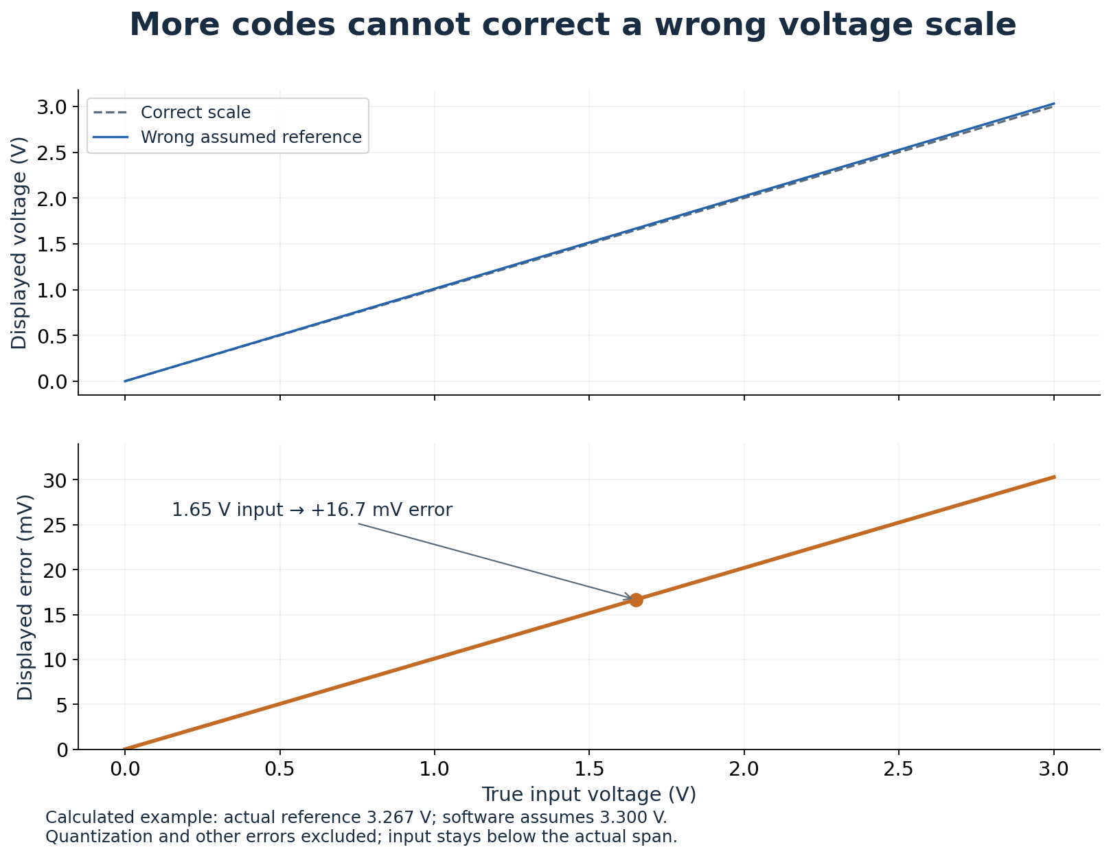
Figure 1. Idealized scale error caused solely by the stated reference mismatch. Quantization, saturation, noise, and other circuit errors are excluded. The calculation stays inside the actual input span.

This is why a stable number can be persuasive for the wrong reason. Imagine taking a hundred readings and obtaining nearly the same value each time. The repetition supports a claim about short-term consistency under those conditions. It does not, by itself, establish agreement with the input voltage. NIST's terminology guidance distinguishes accuracy from precision and treats accuracy as a qualitative concept; numerical statements should specify an appropriate error or uncertainty measure.[2] In practical writing, I want those measures named rather than hidden behind “very accurate.”

There is also a distinction between knowing an error and allowing for uncertainty. In our constructed calculation, the actual reference is stipulated exactly, so we can calculate the scale error. In a real instrument, a reference measurement itself comes with uncertainty and operating conditions. Replacing “3.300” with a newly measured value may improve the conversion while leaving uncertainty in that value. Calibration creates evidence about a relationship. It does not remove the need to describe how well that relationship is known.

One wrong reading can have several contributors

A convenient illustrative model is: reported voltage equals the input multiplied by a scale factor, plus an offset, plus a varying term, plus quantization. This is not a universal circuit equation. It is a way to keep different questions separate. A scale error grows with input magnitude in this simplified model. An offset shifts the reading by a fixed amount. A varying term changes between observations. Quantization restricts the possible output codes. Different experiments are needed to identify these contributions.

Texas Instruments' discussion of total unadjusted error identifies offset, gain error, and integral nonlinearity as distinct features of an ADC transfer characteristic.[3] Offset and gain describe displacement and slope; nonlinearity describes departures that remain beyond a straight-line relationship. The surrounding input driver and reference can contribute too. These distinctions explain why testing one input point cannot establish performance over the whole span. Several very different error curves can cross the same apparently correct point.

Consider two fictional instruments. Instrument A reports every input 5 millivolts too high. Instrument B reports one percent too high. At an input of 0.5 volts, both report 0.505 volts. One test therefore makes them look identical. At 2 volts, A reports 2.005 volts while B reports 2.020 volts. A second point separates the hypotheses. This is a small example, but it captures a general investigative habit: choose a follow-up measurement where competing explanations predict different results.

Two points still do not prove that the response between them is straight. Construct a third instrument that agrees at both calibration points but bows above the line in the middle. A two-point correction removes the endpoint differences while leaving that middle deviation. We would need intermediate checks to detect it. The important question is not how many calibration numbers the software can store. It is which behavior those numbers can represent and whether independent measurements test the behavior left between them.

Temperature adds another experimental axis. Suppose an instrument passes our checks in one controlled condition, then operates elsewhere. We cannot calculate its new error without information about how the relevant components change. A responsible report should preserve the conditions of the original result. “Checked at room temperature” is a narrower claim than “maintains this performance throughout the operating range.” The latter needs evidence across that range or a justified component and system analysis. The same reasoning applies to supply voltage and elapsed time.

Averaging makes some errors smaller

Let us build a second mathematical example. The true input is 1.000 volts. Every reading contains a fixed positive offset of 10 millivolts and independent random noise with zero mean and a standard deviation of 2 millivolts. The expected reading is therefore 1.010 volts. Average a hundred independent readings and the noise standard deviation of that average becomes 0.2 millivolts, because it scales as one over the square root of the number of observations. The 10-millivolt offset remains.

The average looks substantially calmer. It is still centered on the wrong value. This is the situation I would want a dashboard to make visible rather than hide behind extra decimal places. Under our assumptions, averaging improves repeatability of the estimated mean without correcting the stipulated bias. If the random terms are correlated or the input changes while samples are collected, the simple square-root calculation no longer describes the entire problem. The assumptions should travel with the attractive improvement figure.

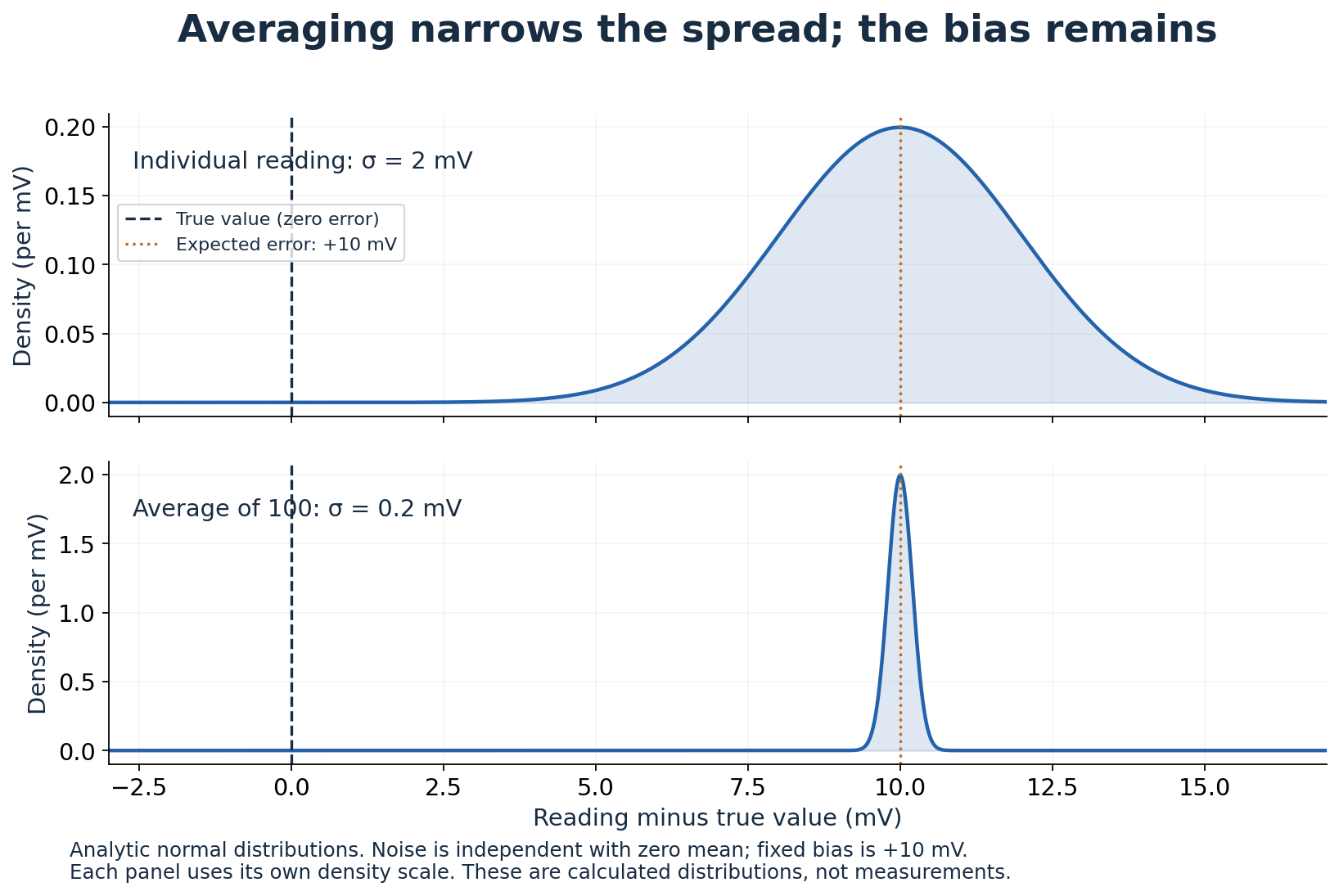
Figure 2. Analytic normal distributions for the constructed example. Single-reading standard deviation is 2 millivolts; the average of 100 independent readings has 0.2-millivolt standard deviation. Both retain the same fixed bias.

Analog Devices' MT-004 discusses digital averaging, input-referred noise, and the distinction between noise-free resolution and other bit-related measures.[4] One particularly useful limit is simple: averaging an unchanged output code returns that same code. Averaging does not conjure variation that was never represented. Appropriate noise and processing can sometimes reveal information about values between nominal code levels, but that result depends on the signal, noise, converter behavior, and arithmetic. It should be demonstrated for the system rather than promised from a slogan.

Averaging also occupies time. If our device collects 1,000 samples per second and forms nonoverlapping groups of 100, it produces ten averages per second. Each group spans approximately a tenth of a second of acquisition. A sudden input change within the group is blended with earlier values. That may be acceptable for a slowly changing quantity and unhelpful for a brief event. The smoother display is the result of a changed observation process, not a free improvement in every dimension of performance.

To see the consequence without a circuit, imagine a group containing fifty readings at 1 volt and fifty at 2 volts. Its average is 1.5 volts. No individual reading needs to have been 1.5 volts. A user looking only at the average could mistake a sharp transition for an intermediate state. This example does not make averaging undesirable. It makes the question precise: are we estimating a stable mean, following a transition, or trying to detect a short excursion? Each task values the lost timing information differently.

ENOB answers a different question

Effective number of bits, usually abbreviated ENOB, is another specification that can sound more general than it is. Analog Devices' MT-003 relates ENOB to signal-to-noise-and-distortion ratio, or SINAD, for a dynamic test with a specified input.[5] In the full-scale sine-wave form, ENOB is approximately (SINAD − 1.76)/6.02. That connects the measured dynamic result to an ideal converter comparison. It does not say that every DC voltage is correct to that many binary digits.

For example, a hypothetical full-scale sine-wave test yielding 68 decibels SINAD corresponds to approximately eleven effective bits by that formula. The calculation could describe a converter whose output word contains sixteen bits. There is no missing packet of five bits. The nominal code space and the dynamic performance measure describe different aspects of the device. The input frequency, amplitude, sampling rate, and measurement bandwidth matter when comparing ENOB values; a result under one set of conditions cannot automatically stand in for another.

This is where I would slow down when comparing two data sheets. If one prominent number was measured with a low-frequency input and another with a much higher-frequency input, ranking them without reading the conditions could reward the easier test. Likewise, a filtered result and an unfiltered result may cover different noise bandwidths. The comparison should begin with the task's operating conditions. A spreadsheet of headline numbers becomes useful only after the rows describe comparable measurements.

Build the test around the actual question

Suppose the project is a battery monitor that needs to recognize a change of 10 millivolts over several seconds. I would first state that requirement, the input range, the expected temperature range, and the allowed delay. Then I would examine the entire path that converts the battery voltage into the ADC input and then into the displayed value. A resistor divider, for example, introduces a conversion ratio that software must know. Testing the converter alone would leave that ratio outside the evidence.

For an illustrative divider calculation, assume software expects the ADC input to be exactly one quarter of the measured voltage. An ADC reading of 1.000 volts becomes a displayed 4.000 volts. If the actual divider ratio is instead 0.2525, a true 4.000-volt input produces 1.010 volts at the converter and a displayed 4.040 volts. The converter could be ideal and the overall result still wrong. This is another scale error, introduced before the part whose bit count often receives all the attention.

The test should therefore include known inputs at the system boundary, not only at an internal pin. I would compare repeated readings at several points, record operating conditions, and reserve additional points for checking the correction. The reference instrument's uncertainty must be suitable for the intended claim. Otherwise the test can establish agreement between two readings without establishing that either supports the required error limit. The point of an independent reference is to add information, not just another impressive display.

I would also examine behavior near the ends of the intended range. A sensor path that works well in the middle may approach a limit elsewhere. If a code remains pinned at its maximum, that output tells us the input has reached a boundary of the represented range; it does not reveal how far beyond the boundary the underlying quantity went. In our idealized model, any larger input after saturation has lost amplitude information. Extra averaging of the maximum code cannot restore it.

Software deserves an equally concrete check. Are signed and unsigned codes interpreted correctly? Does a conversion use the actual configured input range? Is a stored calibration value expressed in volts or millivolts? These are questions to test against the implementation, not accusations about a particular product. A useful end-to-end check applies a known physical input and follows the resulting value through each conversion. Finding where the value first diverges narrows the investigation much more effectively than replacing the most expensive component first.

A correction needs a separate check

Here is a complete small calibration example. Suppose a fictional instrument reports 0.507 volts when presented with 0.500 volts, and 2.017 volts when presented with 2.000 volts. Assume for this calculation that both reference inputs are exact and the response is linear. The reported change is 1.510 volts for an actual change of 1.500 volts, so the fitted scale factor is about 1.006667. Substituting either point gives a fitted offset of approximately 3.667 millivolts.

To correct a later report under that model, subtract the fitted offset and divide by the fitted scale factor. A report of 1.262 volts then becomes 1.250 volts. That is a useful calculation, but applying it to the two points used to construct the correction is not an independent demonstration of success. The model was built to fit them. I would apply additional reference inputs, including the intermediate 1.250-volt point, and examine the remaining differences without refitting the model to each result.

Now relax the convenient assumption that the reference inputs are exact. Their uncertainties contribute to uncertainty in the fitted slope and offset, and therefore to the corrected reading. Repeated observations may help estimate some varying contributions, while other contributions require calibration records or a justified model. The correction can still improve the measurement. It simply needs a report that distinguishes the estimated adjustment from the confidence placed in the adjusted value. Publishing six decimal places does not perform that analysis for us.

Report enough detail to make the number useful

A useful result might say that, over a stated range and set of conditions, the system's readings differed from the reference by specified amounts, with a documented uncertainty analysis. It would identify the averaging interval and any correction applied. That description is less compact than “16-bit accurate,” but it lets another person assess whether the measurement suits their task. It also makes later changes visible. Replacing a reference or modifying a filter can then be evaluated against a defined baseline.

I would keep raw codes alongside converted values during development when practical. That makes it possible to distinguish a changing input code from a changing scale factor in software. It also helps reveal whether a smooth output is created by filtering rather than by a quiet acquisition path. The retained record should include configuration, units, and timing. A column of numbers without those details can be difficult to interpret later, even when every number was stored without corruption.

The final purchase decision should follow the investigation. If quantization is limiting the required discrimination, additional resolution may be exactly what the project needs. If the dominant error is the reference or divider ratio, addressing that relationship may provide more benefit. If the task needs faster response, a heavily averaged result may be the wrong trade. The question is which change improves the specified measurement, not which component offers the longest output word.

More bits are useful when the rest of the measurement lets us use them. They give us finer possible distinctions, but they do not establish that the ruler is correctly scaled or that the reported quantity matches the thing we intended to observe. I want the extra digits to be supported by that chain of evidence. Otherwise we have made the display more precise while leaving the most important uncertainty untouched: whether the number means what the reader thinks it means.

References and method

1. Walt Kester, Analog Devices, MT-001: Taking the Mystery out of the Infamous Formula, SNR = 6.02N + 1.76 dB; ideal quantization model and its assumptions.
2. NIST, Technical Note 1297, Appendix D1: Terminology; accuracy, precision, and uncertainty terminology.
3. Texas Instruments, ADC Accuracy Part 2: Total Unadjusted Error Explained; offset, gain, and integral nonlinearity. The worked examples here do not assume that worst-case error bounds can generally be combined by root-sum-square.
4. Walt Kester, Analog Devices, MT-004: The Good, the Bad, and the Ugly Aspects of ADC Input Noise; averaging and noise-related resolution measures.
5. Walt Kester, Analog Devices, MT-003: Understand SINAD, ENOB, SNR, THD, THD + N, and SFDR; dynamic performance definitions and test conditions.

All voltages, errors, distributions, and instrument comparisons in the examples are constructed. Figures show calculations under stated assumptions, not measured hardware performance. Sources checked on 3 October 2026.

Explore the complete Signals Around Us series.