What Bandwidth Actually Limits

Someone doubles a channel's width and expects a file to arrive in half the time. The reasoning sounds reasonable: more bandwidth should mean more room for information. Yet the transfer improves only a little, or the connection becomes less reliable. It is tempting to blame the equipment or declare that the specification was misleading. Before doing either, I would ask which bandwidth changed, which other quantities stayed fixed, and where the end-to-end transfer was limited.

The same word is used for a frequency range in hertz and, informally, for a delivery rate in bits per second. Those quantities are related in communication systems, but they are not the same measurement. A channel width describes a spectral resource. A delivered bit rate depends on how that resource is used and on constraints elsewhere. This article follows a set of constructed examples through those distinctions. None is a benchmark of a particular radio, internet service, or optical product.

The central investigation is deliberately narrow: what follows from widening an ideal noisy channel under two different power assumptions? From there, we can separate a mathematical capacity limit from modulation choices, packet delivery, and latency. Shannon's original communication theory supplies the foundation, while later treatments clarify the band-limited Gaussian model.[1][2] The useful result is not one universal conversion factor between hertz and bits. It is a way to ask what a bandwidth claim actually promises.

Specify the frequency range before discussing speed

Suppose a hypothetical signal occupies frequencies from ninety-nine to one hundred and one megahertz. The span between those stated edges is two megahertz. The center frequency is one hundred megahertz. These are different properties: shifting the entire signal upward in frequency can change the center without changing that span. A headline saying “higher frequency means more bandwidth” therefore needs an additional argument about the available spectrum or system design. The arithmetic alone does not establish it.

Even spectral width needs a definition. A filter's passband, a signal's occupied bandwidth, an allocation, and a receiver's noise bandwidth describe related but distinct boundaries. A signal can have small spectral contributions outside a nominal edge, while a filter does not necessarily stop everything at one exact frequency. I would read the measurement convention attached to the number. Otherwise two specifications can disagree numerically while describing different aspects of the same system.

To keep our examples unambiguous, let B mean the bandwidth used in a specified ideal additive white Gaussian noise channel model. Let S be average received signal power and N be noise power integrated over that same bandwidth. The capacity expression will use those definitions consistently. This abstraction leaves out fading, practical spectral masks, hardware limitations, and many other effects. Those omissions do not make the calculation useless; they define the narrower question it can answer.

Count distinguishable choices, not merely oscillations

A carrier can oscillate millions of times per second without carrying millions of independent new decisions. Information is conveyed through distinguishable changes selected by an encoding scheme. A symbol might select one of four allowed states, for example. If those states represent equally sized binary labels, each symbol label contains two bits. Sixteen allowed states can label four bits. This counting describes the labeling scheme; it does not prove that a noisy receiver can distinguish every selected state reliably.

In a constructed system sending one million four-state symbols per second, the uncoded labels contain two million bits per second. Change to sixteen states at the same symbol rate and the gross label rate becomes four million. The waveform's spectral requirements depend on pulse shaping and the modulation arrangement. It is therefore incomplete to infer bit rate from bandwidth without specifying the signaling method. More labeled choices per symbol can increase the rate while making the discrimination problem harder under fixed resources.

Coding adds another layer. If only three quarters of a coded bit stream represents the original information in our hypothetical accounting, a four-megabit coded stream carries three megabits of information per second before other overhead. That reduction is not necessarily waste: redundancy can improve reliable recovery. The sensible comparison is successful delivery under stated error and delay requirements, rather than the largest number obtained by multiplying a symbol rate by a label size.

Read the capacity formula as a conditional statement

For the ideal channel under discussion, the familiar expression is C = B log2(1 + S/N), with C in bits per second when B is in hertz and S/N is a linear power ratio. The ratio inside the logarithm is not a decibel value. Ten decibels corresponds to a linear ratio of ten; twenty decibels corresponds to one hundred. Inserting the displayed decibel number directly can produce a plausible-looking but incorrect result. Our decibel article explains that conversion in detail.

Take B as one megahertz and S/N as ten. The calculated capacity is approximately 3.459 megabits per second. This number belongs to the idealized statistical channel, not to an unspecified network connection. Capacity characterizes the boundary for reliable communication in the relevant coding limit. It does not promise that a short packet, a particular code, or a low-cost receiver will achieve that rate with the desired delay and error probability.

The formula is still useful for challenging assumptions. If a proposed system claims arbitrarily high reliable information rate while bandwidth and received signal-to-noise ratio remain fixed in this model, something in the claim needs explanation. Perhaps the model is inappropriate, perhaps more independent channels are involved, or perhaps the quoted rate counts something other than recovered information. A physical limit is most helpful when its conditions are visible enough to compare with the proposed system.

Doubling width while holding the ratio fixed

First, double the bandwidth from one to two megahertz and stipulate that S/N remains ten. The formula doubles capacity to approximately 6.919 megabits per second. The logarithmic factor is unchanged, so the bandwidth multiplier doubles the result. This is the clean version of the intuition that a wider channel gives proportionally more capacity. But the phrase “ratio remains ten” carries a resource assumption that cannot be silently carried into every practical comparison.

If noise power per hertz remains constant, doubling bandwidth doubles integrated noise power. Maintaining the same signal-to-noise ratio then requires twice the average received signal power in this model. Our first calculation has therefore changed both bandwidth and the required signal power relative to that constant noise density. It is valid as a conditional comparison. It is misleading if presented as the guaranteed benefit of changing only one bandwidth setting while all other resources remain fixed.

This is the question I would put beside any impressive before-and-after result: what was held constant? Total transmitted power, received power, power per hertz, antenna configuration, noise density, and error target are not interchangeable controls. A comparison can be internally correct and still answer a different question from the one the reader assumes. Writing down the controls often reveals the disagreement before anyone needs a more elaborate simulation.

Doubling width while holding total power fixed

Now repeat the experiment with fixed average received signal power and fixed white-noise density. At one megahertz, choose their relationship to give S/N equal to ten. At two megahertz, the noise power doubles while the signal power stays constant, so the ratio falls to five. Capacity becomes 2 log2(6), approximately 5.170 megabits per second. The increase is substantial, but it is about 49.5 percent rather than one hundred percent.

At four megahertz, the ratio falls to 2.5 and capacity becomes approximately 7.229 megabits per second. We have gained another two megahertz but a smaller increment in capacity per added megahertz. The calculation is not saying that wider channels are pointless. It shows diminishing returns under the particular fixed-power assumption. The competing fixed-ratio calculation follows a different curve because it supplies different resources as the bandwidth changes.

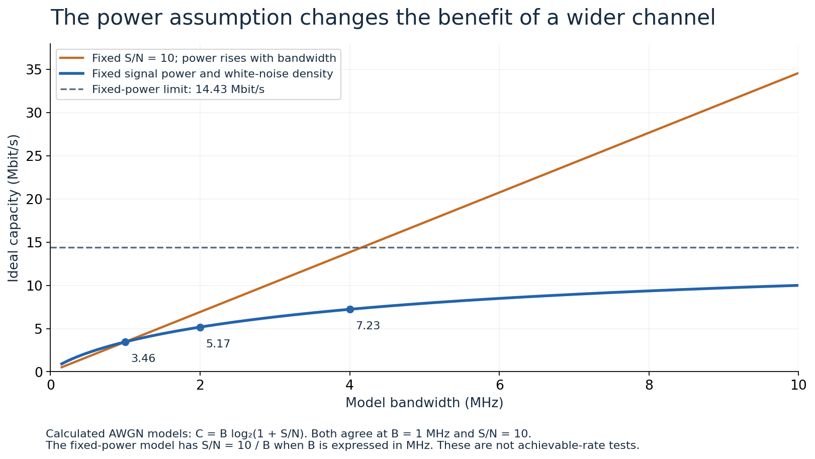
Figure 1. Both models start at 1 MHz and a linear signal-to-noise ratio of 10. The fixed-ratio curve requires increasing signal power as bandwidth grows when noise density is fixed. The fixed-power curve approaches a finite limit. These are mathematical models, not product performance measurements.

Writing the fixed-power expression as B log2(1 + A/B), where A represents signal power divided by the specified noise-power density, makes the trend clearer. In this example A is ten million hertz. As B becomes very large, the expression approaches A divided by the natural logarithm of two, approximately 14.427 megabits per second. An unlimited frequency span does not create unlimited capacity under these particular fixed-power and white-noise assumptions. Changing the assumptions changes the conclusion.

The real channel may not improve smoothly

An actual receiver operates with supported modulation and coding choices, practical estimation, and finite processing. Its measured delivery rate can change in steps rather than tracing a smooth theoretical curve. A wider setting may encounter frequency-selective interference or portions of the channel with different quality. Those possibilities are reasons to measure the system, not reasons to discard the ideal model. The model identifies one relationship; implementation and environment determine how closely a particular link follows it.

Suppose a fictional test gives a higher gross bit rate but more retransmissions after widening the channel. I would compare successfully delivered payload over the same time interval, alongside error counters and the selected coding mode. The gross rate alone might exaggerate the improvement. Conversely, a lower gross rate with far fewer failed transmissions could deliver more useful data. The relevant result depends on the application's accounting boundary, especially when latency or deadline misses matter.

Repeated tests should also control the offered load and the observation period. A lightly loaded source cannot demonstrate the maximum delivery capacity of a link, while a changing source can make a stable link look variable. Record what was sent, what arrived, and when. If interference or fading varies, preserve that variation instead of presenting a single favorable run as a universal property. A measurement becomes more useful when its conditions can be reproduced or at least compared explicitly.

A path can be narrower than its fastest link

Move from the radio model to a fictional packet path with successive link capacities of one hundred, twenty, and one hundred megabits per second. Under a simple steady-flow model, the middle link limits the path to twenty before considering other traffic and overhead. Upgrading the first link to a thousand does not remove that bottleneck. This is why an application's transfer speed is not an independent measurement of the access radio's spectral capability.

RFC 5136 distinguishes link capacity, path capacity, utilization, and available capacity, with explicit attention to packet type and measurement interval.[3] In a constructed example where the twenty-megabit link is already using half its capacity for other traffic under the chosen definition, the available amount is ten megabits per second. It is not necessarily the amount a new application will receive: scheduling, transport behavior, and other constraints still matter. The distinction prevents an available-capacity estimate from becoming an unconditional service promise.

I would therefore locate a suspected bottleneck before recommending a bandwidth change. Compare observations at appropriate boundaries and check whether the sender, receiver, or another shared link is limiting delivery. A fast local test and a slow remote transfer are compatible if they traverse different constraints. The conclusion should identify what was actually tested. Calling both results “the bandwidth” erases the information needed to understand why they differ.

Payload accounting changes the reported rate

Imagine a deliberately simplified transmission unit containing one thousand bytes of useful application data and one hundred bytes of all other accounted material. If a stream delivers these units without loss at eleven megabits per second at that accounting boundary, useful payload arrives at ten megabits per second. The extra bytes have not disappeared; they serve whatever framing, control, or protection the fictional format defines. This example does not claim those overheads for Ethernet, Wi-Fi, or any other named protocol.

Now suppose some units must be sent again. The transmitted bit count can rise without an equal increase in newly delivered application data. If a dashboard counts all transmission attempts while another counts unique received payload, their rates can diverge. Both numbers may be correct for their definitions. An investigation should preserve those definitions rather than resolving the disagreement by choosing whichever display appears more authoritative or gives the more satisfying number.

Compression introduces a different accounting change. A highly compressible input can represent more original application bytes than the number of bytes actually transmitted. That does not violate a channel-capacity result whose information model and boundary differ from the file-size label. I would state whether a reported transfer rate counts original bytes, compressed bytes, coded bits, or physical transmissions. Without that distinction, demonstrations can make ordinary representation changes look like extraordinary communication performance.

More capacity does not remove every delay

Consider a constructed 1,500-byte packet, ignoring additional framing for this calculation. It contains twelve thousand bits. Serializing those bits takes twelve milliseconds at one megabit per second, 1.2 milliseconds at ten megabits, and 0.12 milliseconds at one hundred megabits. Increasing the rate greatly reduces this component of delay. It does not, by that arithmetic alone, change propagation time, processing time, or a fixed waiting period elsewhere in the application.

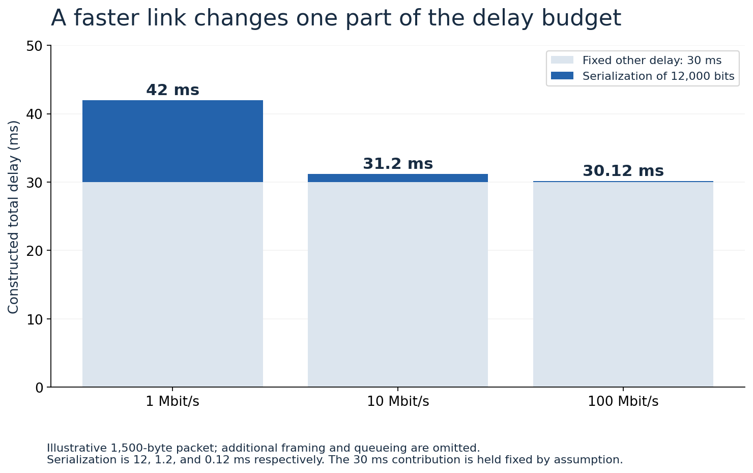
Figure 2. The constructed totals are 42, 31.2, and 30.12 milliseconds. Only serialization changes in this example. The fixed 30 milliseconds is an explicit modeling assumption, not a measured internet round-trip time.

Add a fixed thirty milliseconds from all other modeled contributions. Total delay becomes forty-two, 31.2, and 30.12 milliseconds respectively. The tenfold rate increase from ten to one hundred megabits saves only 1.08 milliseconds in this example. A user expecting every operation to become ten times faster would be disappointed, even though the serialization improvement is exactly as predicted. The task is to identify which parts of the operation the upgraded resource can actually affect.

Queueing can change the picture again. If a link is overloaded, increasing its service rate may reduce waiting substantially. But that benefit depends on the arrival process and the queue's behavior; it is not captured by our fixed-delay illustration. For an interactive voice system, I would examine delay variation and deadline misses as well as average delivery rate. A high-throughput connection can still provide poor conversational experience if the relevant packets wait too long.

Solve the equation backward before choosing a design

The same capacity expression can test an ideal requirement from the other direction. Suppose a proposed information rate is four megabits per second in a one-megahertz channel. The required ratio at the capacity boundary is 2 to the power of four, minus one: fifteen in linear units, or approximately 11.76 decibels. That is a mathematical boundary under the stated model, not a sufficient receiver specification. A practical design would need its own coding, implementation, and reliability analysis.

Keep the four-megabit target but allow two megahertz. The boundary ratio becomes 2 squared minus one, or three, approximately 4.77 decibels. The lower required ratio explains one way bandwidth can substitute for signal quality. It does not mean the required absolute received power falls by the same decibel difference when noise density is fixed, because the wider band contains more noise. Multiplying the ratio by the integrated noise is necessary before comparing the corresponding signal powers.

For a purely numerical noise density of one arbitrary power unit per megahertz, the narrow model contains one unit of noise and requires fifteen units of signal power at that boundary. The wider model contains two units of noise and requires six units of signal power. The example exposes both calculations explicitly. A comparison based only on the ratios would miss the bandwidth-dependent noise term. A comparison based only on the bandwidth would miss the changed reliability requirement.

Shared airtime introduces a different constraint

Imagine two independent application flows sharing one hypothetical transmitter that can send only one of their frames at a time. If the system gives each flow half of the usable transmission time, neither receives the transmitter's full continuous payload rate. That sharing is a scheduling fact, separate from the frequency width. It remains relevant even when every transmitted frame is decoded perfectly. A larger physical capacity can help, but it does not erase the distinction between total shared capacity and one participant's allocation.

Now add a fictional control interval occupying ten percent of the schedule. Of the remaining ninety percent, divide time equally between the two flows. Each receives forty-five percent of the original transmission opportunity under this deliberately simple model. At a twenty-megabit payload rate during its active periods, each averages nine megabits per second. These numbers are an accounting example, not an assertion about the scheduler or overhead of any wireless standard.

Bursty applications make average allocation an incomplete experience measure. Two schedules can deliver the same nine-megabit average while providing very different gaps between opportunities. One might suit a large file better than an application with short deadlines. I would preserve the distribution of waiting times, not merely the total bytes delivered. This is especially relevant when evaluating communication as a service to a person, because a successful eventual transfer does not guarantee a timely response.

The broader point is that a resource can be sufficient in aggregate and still be unavailable at the moment a particular packet needs it. To investigate that failure, record queue arrival times, service opportunities, and completion times at the relevant boundary. Those observations test a scheduling explanation directly. Increasing spectral width without measuring them may improve the symptom, but it would leave the underlying account of why the delay occurred incomplete.

Turn the claim into a testable question

For the original complaint, I would write the claim in measurable terms: widening this channel, with these power settings and this traffic, should improve unique payload delivery by a stated amount over a defined interval. Then preserve the signal-to-noise measurements, selected modes, errors, competing traffic, and end-to-end timing. That makes a disappointing result investigable. “The wider setting was bad” provides almost none of the information needed to separate channel conditions from a bottleneck elsewhere.

The next measurement should distinguish competing explanations. If the local link improves but the remote transfer does not, inspect the rest of the path. If received signal quality changes with width, examine the power and noise assumptions. If gross rate rises while useful delivery falls, inspect errors and overhead. These are diagnostic branches, not a universal troubleshooting sequence. Their purpose is to connect each proposed explanation to an observation that could support or weaken it.

Bandwidth matters because communication requires physical and temporal resources. It becomes misleading only when one resource is made to stand for the entire system. Hertz, gross bits, recovered information, unique payload, and response time answer different questions. A defensible account follows the relationships between them, states what remained fixed, and leaves the reader able to repeat the calculation. That is how a wider channel becomes a specific engineering claim rather than a vague promise of speed.

References and method

1. Claude E. Shannon, A Mathematical Theory of Communication, 1948; foundational communication and capacity results.
2. Nokia Bell Labs, The Capacity of the Band-Limited Gaussian Channel; statement of the Gaussian channel model and coding boundary.
3. IETF, RFC 5136: Defining Network Capacity; network-layer capacity, utilization, and available-capacity definitions.

All numerical links, powers, overheads, and delays are constructed. Capacity figures are direct calculations from the stated ideal model; they are not measured achievable rates. Decimal prefixes are used for megahertz and megabits per second. Sources checked on 3 October 2026.

Explore the complete Signals Around Us series.