Aliasing and the Apparently Backward Wheel

A wheel turns forward, yet the recording seems to show it turning backward. The vehicle has not suddenly discovered a different law of motion. Something happened between the moving object and the sequence we are watching. That gap is where I want to start. A camera records observations separated in time. We supply a story about the motion between them. Usually the story feels effortless. Sometimes the observations allow more than one story, and the one that looks most obvious is wrong.

This is a useful problem because it does not stay inside a camera. A vibration monitor can report a frequency that was not the original vibration. A recorded tone can emerge at a lower pitch. A plotted sensor trace can look smooth while concealing fast changes between its points. The shared issue is aliasing: different underlying variations can produce the same sampled observations. The recording can be internally consistent, repeatable, and beautifully displayed while remaining insufficient to identify what actually happened.

We can investigate the problem without relying on a dramatic video or an undocumented experiment. The examples below are constructed, and the diagrams are calculated from the stated numbers. That gives us an advantage: we know the motion or waveform before sampling it. We can compare the original with what survives observation. In a field investigation, establishing that original would be part of the work. Here, deliberately controlling it lets us locate the ambiguity rather than merely suspect it.

Follow one mark around the wheel

Imagine a disk with one clearly identifiable mark on its rim. Assume the camera takes instantaneous, evenly spaced frames at 24 frames per second. Now let the disk turn forward at 23 revolutions per second. Between consecutive frames it completes 23/24 of a revolution, or 345 degrees. The mark therefore appears 345 degrees farther forward. But the same visible position is also 15 degrees backward from the previous one. The camera has recorded a position; it has not recorded which route the mark took to reach it.

Follow the smaller displacement through 24 frames and the mark seems to complete one backward revolution each second. In this ideal example, a disk moving forward at 23 revolutions per second and one moving backward at one revolution per second have identical recorded orientations at every frame time. This is stronger than saying the pictures look approximately alike. Given the assumptions, their sampled orientations are exactly alike. More careful inspection of those same positions cannot recover the missing turns.

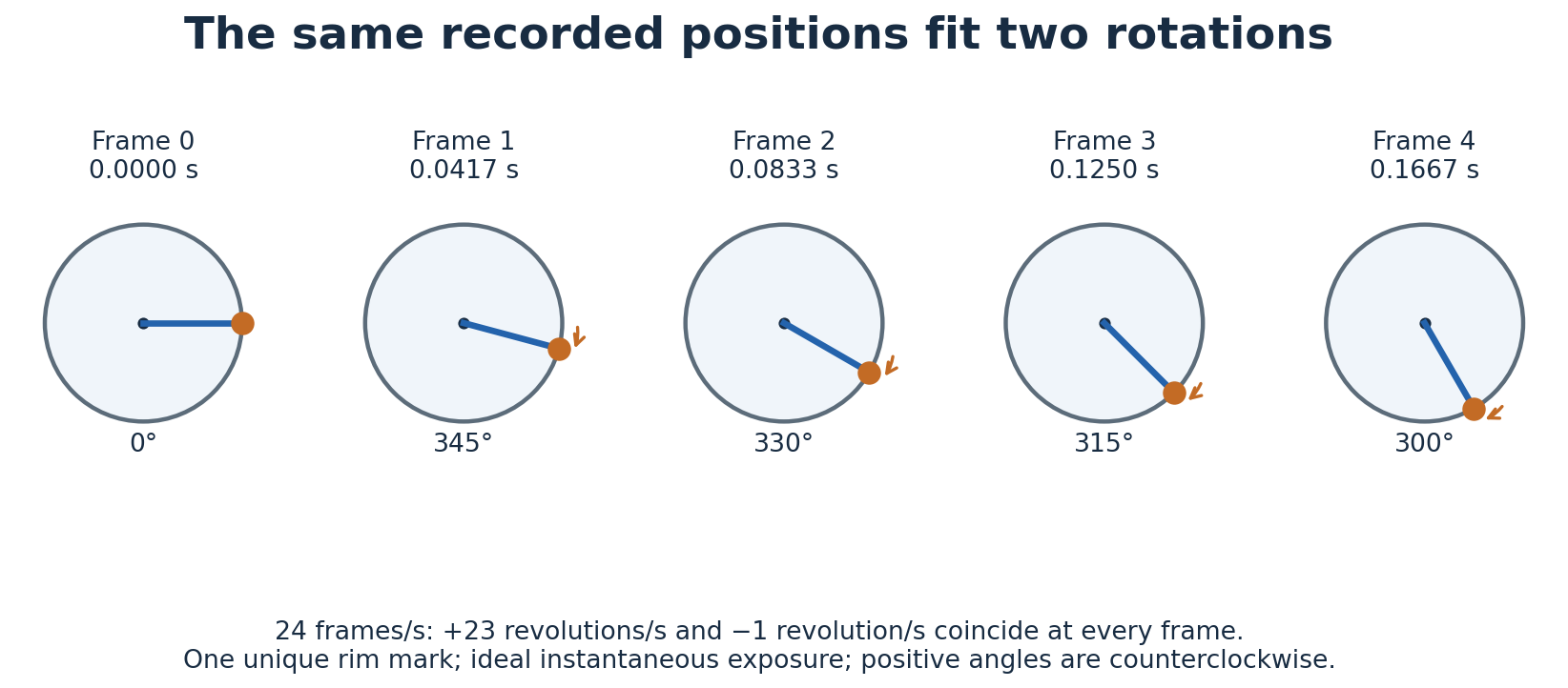
Figure 1. Calculated orientations for an ideal disk with one unique mark. The arrows show the short apparent movement between frames; the unrecorded forward movement is 345 degrees per frame. Exposure duration is assumed negligible.

The unique mark matters. A real wheel may have several visually identical spokes. If eight spokes are evenly spaced, rotating it by 45 degrees returns the same pattern. The image then repeats eight times per mechanical revolution. Confusing those repetitions with complete revolutions introduces another ambiguity. Before estimating speed from a repeating object, I would ask what feature is being tracked and how many indistinguishable copies exist. “The wheel moved one position” is not a measurement until “position” has a defined meaning.

For a second invented example, let an eight-spoke wheel rotate at 2.75 revolutions per second under our 24-frame camera. The spoke pattern passes a fixed orientation 22 times per second. Between frames, the wheel moves 41.25 degrees forward. Because the pattern repeats every 45 degrees, the same frame-to-frame pattern can be explained by a movement of 3.75 degrees backward. That corresponds to an apparent backward speed of 0.25 revolutions per second. The physical speed and the rate at which a repeated pattern presents itself are different quantities.

MIT's sampling lecture connects this ambiguity with stroboscopic demonstrations of rotating and oscillating objects.[1] The important observation is that the sampling can come from intermittent illumination as well as from a camera. If an object is visible only at particular instants, its motion between those instants remains unobserved. Our wheel calculations are an explicit version of that idea. They are not a claim about the frame rate, exposure, illumination, or construction of any particular circulating video.

Two different waves leave the same evidence

Now replace the disk with an electrical signal. We sample a cosine wave 100 times per second, so adjacent samples are 0.01 seconds apart. Consider one wave at 30 hertz and another at 70 hertz, with equal amplitude and the same cosine starting phase. The first completes 0.3 cycles between samples; the second completes 0.7. At the sample times, their values are identical. Between the sample times, the curves differ substantially. A recorder that retains only those values cannot distinguish the two inputs.

The arithmetic is short enough to inspect. At sample number n, the two values are cos(2π × 30n/100) and cos(2π × 70n/100). Because 70 equals 100 minus 30, the second expression becomes cos(2πn − 2π × 30n/100). An integer number of full turns does not change a cosine, and cosine has the same value at positive and negative angles. The second expression therefore equals the first for every integer n. No random noise, faulty cable, or rounding error is required.

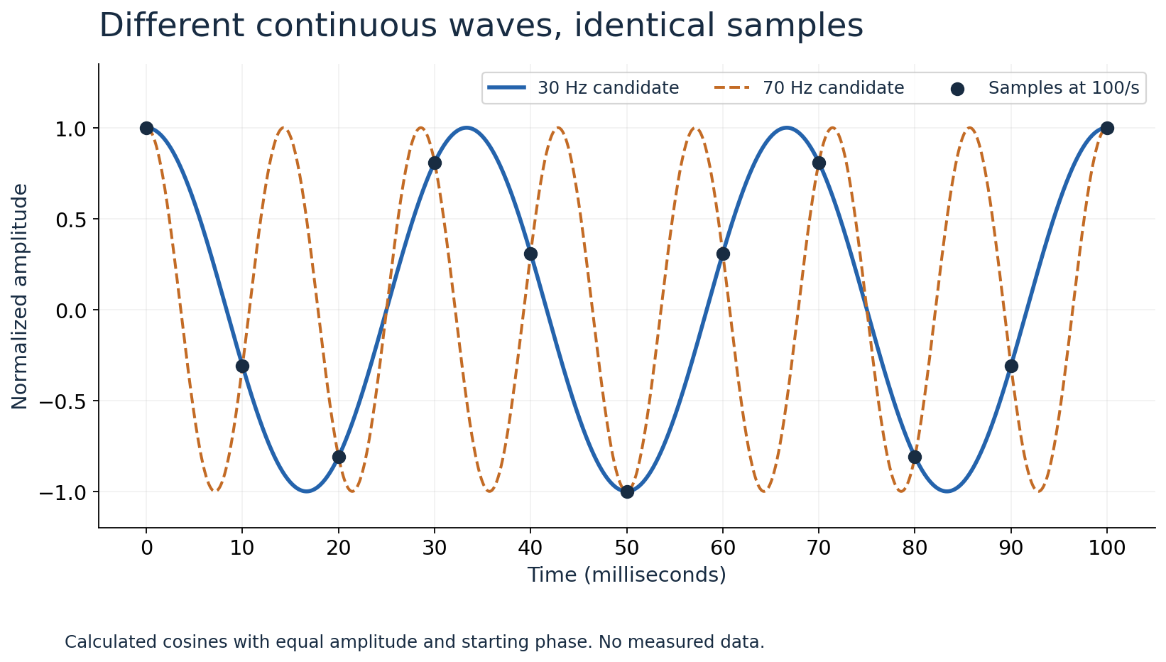
Figure 2. Both calculated waves pass through the black sample points. Amplitude is normalized; the sampling interval is 10 milliseconds. The connecting curves represent two possible inputs, not information stored in the samples.

This distinction changes how I read a plotted line. Software often connects measured points because a continuous trace is easier to follow. But the connecting line is a rendering choice. Unless the acquisition conditions justify a particular reconstruction, it is not an observation of everything between the points. A smooth curve can encourage confidence precisely where the measurement contains a gap. The right question is not whether the line looks plausible. It is whether other physically possible inputs would produce the same recorded data.

A longer recording does not resolve our particular ambiguity. Record ten samples, a thousand samples, or a million samples at exactly the same rate: the ideal 30-hertz and 70-hertz cosines still agree at every sampled instant. More observations help only if they add relevant information. Repeating an ambiguous observation for longer can strengthen the wrong interpretation if the acquisition assumptions remain unexamined. That is why I would inspect the sampling arrangement before celebrating the apparent stability of a suspicious spectral peak.

What the sampling theorem actually promises

MIT's lecture notes state the familiar reconstruction condition for a band-limited signal: equally spaced samples can determine it when the sampling rate exceeds twice its highest frequency.[2] The qualification does essential work. We need a justified limit on the frequencies entering the sampler. The theorem does not say that any unknown physical process becomes fully known once a device reports a nominal sample rate. It connects a mathematical signal class, an observation process, and a reconstruction procedure under specified assumptions.

In the 100-sample example, half the sampling rate is 50 hertz. If we independently know that the input contains no frequencies at or above that boundary, the 70-hertz candidate is excluded. The samples then belong to a much more restricted set of possible inputs. The knowledge of the input bandwidth is doing part of the work. It is not information we discovered solely from the saved numbers. This is why a sampling specification and an input filtering specification belong in the same conversation.

The word “exceeds” also deserves attention. Suppose we sample a 50-hertz sine wave at 100 samples per second, starting exactly at a zero crossing. Each sample lands at another zero crossing. The recorded values are all zero even though the wave changes between them. A cosine at that frequency and a different phase can give alternating values instead. This boundary example explains why merely arranging two observations per cycle is an unsafe practical slogan. Phase and the assumptions at the frequency boundary matter.

Nor is “twice the frequency” a complete purchasing rule. A project needs an acceptable error, a usable frequency range, an input environment, and a realizable filter. These requirements determine what margin is useful. A slow temperature trend accompanied by electrical interference is not the same acquisition problem as a clean laboratory tone, even if both projects care about the same low-frequency variation. The quantity of interest may be slow while unwanted signals reaching the converter are much faster. The converter samples the input it receives, not the intention written in the project brief.

A vibration investigation with a false lead

Imagine a fictional monitoring project that saves a vibration signal at 100 samples per second. Its spectrum shows a strong component at 30 hertz. An investigator suggests that a part is oscillating at that frequency. That is a reasonable hypothesis, but our constructed example immediately supplies another: a 70-hertz input can appear in the same place. The plot establishes a pattern in the recorded sequence. Assigning that pattern to a physical source requires evidence about acquisition and the source itself.

One useful follow-up would be a new recording at 120 samples per second while keeping the physical conditions comparable. In our simplified example, a genuine 30-hertz cosine remains a 30-hertz cosine. The 70-hertz cosine instead aliases to 50 hertz. A feature that moves in the predicted way when the sample rate changes is evidence for the aliasing hypothesis. It is not an automatic verdict in a real installation: changing acquisition settings may also change filtering, sensor modes, or processing. Those changes must be recorded alongside the new rate.

Another follow-up would use an independently characterized measurement path with enough bandwidth and sampling margin to examine the suspected 70-hertz component directly. I would want the two measurements taken under comparable operating conditions, with their time intervals documented. If the equipment changed speed between recordings, a moving spectral peak could reflect the machine rather than the sampler. The purpose of the second instrument is to challenge the first interpretation, not merely to produce another graph that agrees after unknown transformations.

There is also a more basic possibility: perhaps the exported file is not the converter's original output. An acquisition device might sample quickly, process internally, and send a reduced stream to a dashboard. A setting called “update rate” may describe screen refreshes, transmitted summaries, or actual samples. These are hypothetical possibilities to check, not interchangeable terms. I would trace the data from physical input to stored rows and identify every stage that changes the time spacing or combines observations.

That trace should distinguish a missing sample from a regularly discarded sample. Our equations assume known, uniform sample times. If a logger drops records unpredictably and an analyst then pretends the remaining rows are evenly spaced, a different error has entered the reconstruction. A timestamp column helps only if its meaning is known: acquisition time, packet arrival time, and database insertion time can describe different events. The investigation needs the timing of the observation relevant to the model, not simply any available clock value.

Filtering has to arrive before the ambiguity

An anti-aliasing filter reduces unwanted frequency content before the sampling step where it would become ambiguous. Analog Devices' MT-002 tutorial explains the relationship between the filter's finite transition band and the selected sampling rate.[3] Real filters do not abruptly pass everything below one frequency and reject everything above it. Their attenuation changes across a range. Faster sampling can create room for that transition, but the required attenuation still depends on the unwanted input and the error the application can tolerate.

Here is a deliberately simple design calculation. Suppose an unwanted tone entering an analog filter has an amplitude of 1 volt, and we want its remaining contribution below 1 millivolt before sampling. That is an amplitude reduction of 1,000 to one, or 60 decibels, using 20 log10 of the voltage ratio under the same impedance convention. The requirement belongs at the unwanted tone's frequency. Calling a filter “low-pass” does not establish that it delivers this reduction at the point where we need it.

The calculation is an illustrative requirement, not a complete filter design. We have not specified the wanted passband, phase response, component tolerances, sensor impedance, or converter loading. Those omissions would matter in hardware. But even this small calculation improves the discussion: it replaces “remove the high frequencies” with an amplitude target at a defined frequency. A filter that reduces the unwanted tone by ten times would look helpful on a graph and still miss our invented requirement by a factor of one hundred.

Once the 70-hertz cosine has become the same digital sequence as the 30-hertz cosine, a digital filter cannot label which of those two inputs created it using that sequence alone. Removing the apparent 30-hertz component would remove a genuine 30-hertz contribution too. External information might help distinguish the cases, but it would be additional evidence. The missing identity is not hidden in a file waiting for sufficiently confident software. This follows directly from the equality of the sample values in our worked example.

Filtering becomes relevant again when reducing an already digital sample rate. Consider a hypothetical recording at 1,000 samples per second that we want to reduce to 100. Simply keeping every tenth point creates a new sampling step. A digital low-pass filter applied before that reduction can suppress components that would alias at the lower rate. The important word is “before.” Processing after the reduced sequence has already combined indistinguishable possibilities cannot recreate their separate histories without further assumptions.

A frequency label can hide several candidates

Our 30-hertz result has more possible parents than the two we have plotted. At 100 samples per second, equal-amplitude cosines at 130 and 170 hertz also reproduce the same sample sequence with the corresponding cosine phase. Adding a whole number of cycles between observations leaves the observed phase unchanged. A spectrum with a peak labelled 30 hertz therefore does not carry a complete list of the possible original frequencies. That list comes from the sampling model and the independently known input constraints.

This offers a useful way to organize an investigation. If interference is suspected near a particular frequency, calculate where it would appear after sampling and compare that prediction with the observed feature. For example, a 110-hertz cosine sampled at 100 samples per second matches a 10-hertz cosine. At 120 samples per second it also matches 10 hertz, although the signed frequency relationship changes. Simply changing the sampling rate once does not always separate the hypotheses. The choice of the new rate should follow a calculation.

Try 128 samples per second for that same constructed 110-hertz input and the apparent cosine frequency becomes 18 hertz. A genuine 10-hertz input remains at 10. This third rate is more informative for that particular pair of hypotheses. I would write these predictions down before taking the new measurement. Otherwise it is easy to reinterpret whichever peak appears as support for the explanation I already prefer. A test is stronger when the competing explanations predict visibly different outcomes in advance.

The calculation also helps distinguish a frequency change from an amplitude change. Two candidate frequencies may land in the same place after sampling while the analog input filter attenuates them differently. If the filter response is independently known and the input amplitude is controlled, that difference may supply additional evidence. But an unknown source amplitude can preserve the ambiguity: a larger high-frequency input could leave the same sampled amplitude after attenuation. Knowing the filter helps; assuming it solves every unknown does not.

A related trap appears when the display contains only a few points across a cycle. Readers sometimes count visible peaks and treat that count as a direct view of the physical process. In our example, the black dots belong equally to two continuous curves, with different numbers of peaks between them. Drawing more pixels between those dots improves the appearance of the chart without adding observations. Increasing display resolution and increasing acquisition rate solve different problems, even though both can make a screen look more detailed.

There is a practical reporting consequence. A statement such as “the recorded sequence contains a component equivalent to 30 hertz at the stated sample rate” preserves what the analysis established. A statement such as “the machine vibrated at 30 hertz” adds a claim about the source. That stronger claim may be fully justified after checking bandwidth, filtering, and independent measurements. I want the report to show that bridge. Otherwise readers cannot tell whether the source was identified or merely assigned the label used by the plotting software.

Why a real video needs more questions

Our wheel model intentionally excludes exposure duration, changing speed, lighting variation, and the details of how a camera reads its image sensor. A real recording may combine several effects. I would therefore resist diagnosing a specific clip from the backward motion alone. First establish the original recording rate rather than merely the playback rate. Then ask whether frames were removed or duplicated during editing, whether the illumination was continuous, and whether the repeating feature was actually unique enough to track.

These are questions about evidence, not a claim that every unusual video uses the same trick. A frame number tells us the order of images; it does not independently establish how much time elapsed at capture. Slowing playback changes how fast the recorded sequence is presented, while changing the capture interval changes what was observed. Confusing those operations can make a visually persuasive demonstration mathematically incoherent. I would keep the acquisition timeline and the viewing timeline separate when explaining what a clip can establish.

The strongest small demonstration is one whose assumptions readers can reproduce. Our cosine example requires only a calculator or a few lines of code: calculate the two cosines at n/100 seconds and compare the results. Tiny differences from floating-point arithmetic should be interpreted as numerical approximation, not as physical information distinguishing the ideal waves. Plotting the continuous formulas between those samples then reveals exactly what the acquisition omitted. The demonstration works because both the observation and the alternative explanation are explicit.

The apparently backward wheel is memorable, but the more consequential lesson appears in less dramatic places. A confident dashboard label, a stable peak, or an attractive interpolated line can conceal a question the data cannot answer. Before deciding that a process is slow, periodic, or moving in a particular direction, I want to know how often it was observed and what other behavior was excluded before recording. The missing intervals are part of the story. A good investigation makes them visible before building a conclusion across them.

References and method

1. MIT OpenCourseWare, Lecture 16: Sampling, Alan V. Oppenheim with Harold Edgerton; sampling and stroboscopic demonstrations.
2. MIT OpenCourseWare, Sampling lecture notes; reconstruction assumptions and ambiguity under undersampling.
3. Walt Kester, Analog Devices, MT-002: What the Nyquist Criterion Means to Your Sampled Data System Design; practical filtering and sampling-rate choices.

The wheel speeds, frequencies, vibration investigation, and filter target are original constructed examples. Figures were calculated from the formulas in the text; they are not photographs or field measurements. Sources checked on 3 October 2026.

Explore the complete Signals Around Us series.