Time and Frequency: Two Views of One Observation

A recording arrives with a screenshot of two sharp peaks. The accompanying explanation sounds settled: two sources are present, their frequencies are known, and the problem has been identified. Then someone asks when the disturbance started. The screenshot cannot answer. Someone else asks whether the two components arrived together or in separate bursts. The same picture is still insufficient. The analysis may be numerically correct while the evidence needed for those questions has been discarded from its presentation.

This is the useful tension between time and frequency. A time trace makes order and duration visible. A frequency representation can expose repetition that is difficult to recognize in the trace. Neither picture is automatically the more scientific one. I want to follow the same constructed observations through both, checking what the transformation preserves, what a particular display omits, and what a finite recording cannot establish. There are no field measurements in the examples below; every waveform is generated from stated assumptions.

The investigation starts with an important distinction. The full discrete Fourier transform is a reversible representation of a finite sequence, within numerical precision and the chosen convention. A screenshot showing only the magnitudes of some coefficients is a reduced product. The transform did not necessarily destroy the information; the display may have left it out. SciPy's official Fourier tutorial defines the forward and inverse mappings explicitly.[1] Keeping those two operations separate prevents several common misunderstandings.

Begin with the observation we actually have

Imagine a voltage recording sampled at one thousand samples per second. It contains one thousand samples, indexed from zero through nine hundred and ninety-nine. The usual Fourier analysis interval is one second: sample count divided by sampling rate. The timestamp of the final sample is 0.999 seconds, which does not make the interval 0.999 seconds in this convention. That small distinction matters when software builds its frequency axis from the record length. A one-sample bookkeeping error can become a systematic frequency error.

Let the constructed voltage be a fifty-hertz sine wave with a one-volt peak amplitude, plus a one-hundred-and-twenty-hertz sine wave with a 0.4-volt peak amplitude. The trace is the sum, not two separate tracks waiting to be discovered. At each sampling instant, we store one number containing both contributions. Because we specified the components ourselves, we know the answer in advance. That makes this a useful controlled test of analysis conventions, rather than evidence that an unknown machine contains those exact sources.

Before transforming any real record, I would preserve its units, timestamps, sample rate, acquisition settings, and any missing-data markers. A Fourier routine operates on the supplied sequence; it does not know whether the numbers came from volts, pressure, acceleration, or an incorrectly scaled export. A plausible spectrum can be produced from an implausible acquisition. The first question is therefore whether the stored record faithfully represents the intended observation, including the time axis that gives every computed frequency its physical meaning.

A spectrum asks how much of each pattern is present

The discrete transform compares the finite sequence with a family of complex oscillatory patterns. Each coefficient has a magnitude and a phase. In our one-second example, the ordinary transform grid has one-hertz spacing, so both constructed frequencies fall on grid points. With an appropriate amplitude normalization, the positive-frequency display recovers peaks of one volt and 0.4 volts. This agreement is a check on the calculation because we know what we generated. It is not an independent discovery about the world.

For this particular unwindowed, real-valued example, the positive-frequency sinusoidal peak amplitudes can be obtained by multiplying the corresponding transform magnitudes by two and dividing by the sample count. The zero-frequency term and the Nyquist term require different treatment; neither has a distinct negative-frequency partner to combine. Other normalization conventions are equally legitimate if stated consistently. I would never compare two amplitude plots until I knew whether each represented peak amplitude, RMS amplitude, power, or some other quantity.

The spectrum makes the two repetitions easier to see than the original trace. But it does not establish that two physical devices generated them. One nonlinear system can produce multiple spectral components, and several physical sources can contribute at one frequency. Our example contains two mathematical sinusoids because we defined it that way. In an investigation, the statement “there are two spectral peaks” is an observation; “there are two faulty components” is a causal claim that needs additional evidence.

The missing phase changes the story

Now generate a second record with the same two frequencies and amplitudes, but shift the phase of the one-hundred-and-twenty-hertz component by a quarter cycle. The time trace changes. Peaks line up differently, and the instantaneous sums differ. Yet the magnitude spectrum remains the same at the two frequencies. A report containing only those magnitudes cannot distinguish the records. The phase information is present in the complex transform, but absent from that report.

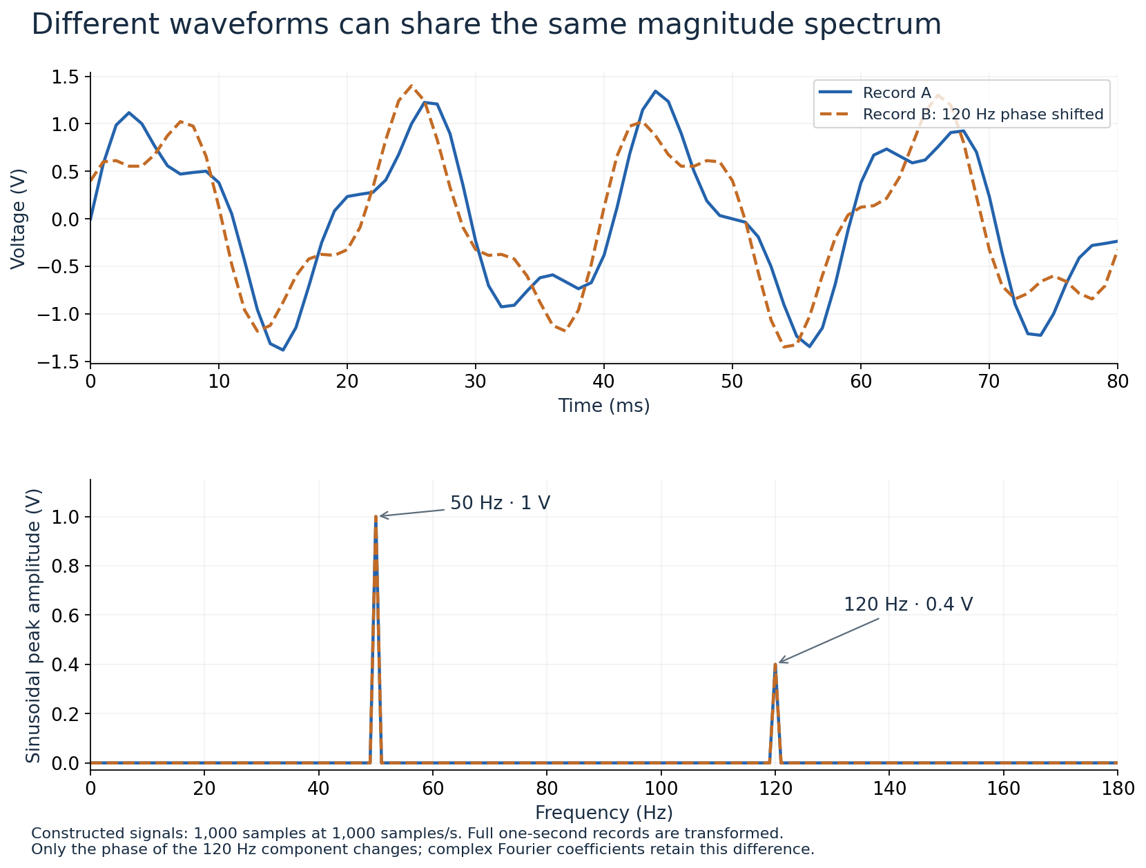
Figure 1. Both records contain the same sinusoidal amplitudes and frequencies. Changing one component's phase changes the waveform while preserving its spectral magnitudes. The first 80 milliseconds are shown above; spectra use the complete one-second records.

MIT's treatment of Fourier-transform properties includes the relationship between time shifts and phase.[2] A delay does not need to change the magnitude spectrum of a fully retained signal to change when it occurs. That makes phase indispensable when reconstructing waveforms or comparing timing between channels. It also explains why a frequency-magnitude display should not be treated as a complete substitute for the original recording. Its usefulness depends on the question, not on how clean its peaks look.

There is a boundary to that statement. Moving a finite event partly outside a fixed observation window changes which samples are retained, so the resulting magnitude spectrum can change as well. “A delay changes phase” assumes the relevant transformed signal and boundary conditions are handled consistently. I would check the captured interval before invoking the rule. Otherwise a real difference in what was recorded can be misdescribed as a contradiction in the mathematics.

More plotted points do not create a longer observation

Consider a harder constructed case: two equal-amplitude tones at fifty and fifty-three hertz. Record only a tenth of a second at the same sampling rate. There are one hundred observed samples, and the ordinary transform grid is ten hertz apart. We can append zeros and compute a transform with thousands of output points. The plotted curve becomes smoother. We have not listened for longer, measured any new samples, or supplied the missing evidence about what happened outside that tenth of a second.

Zero padding evaluates the finite record's spectral representation on a denser frequency grid. It can help locate the shape of a peak and support an estimator, but it does not provide the resolving power of a genuinely longer observation. MIT's notes connect the ability to distinguish nearby components with the observation window and its spectral width.[3] Bin spacing and practical resolution are related concepts, but they are not interchangeable definitions. Resolution also depends on the window, relative amplitudes, noise, and the estimation method.

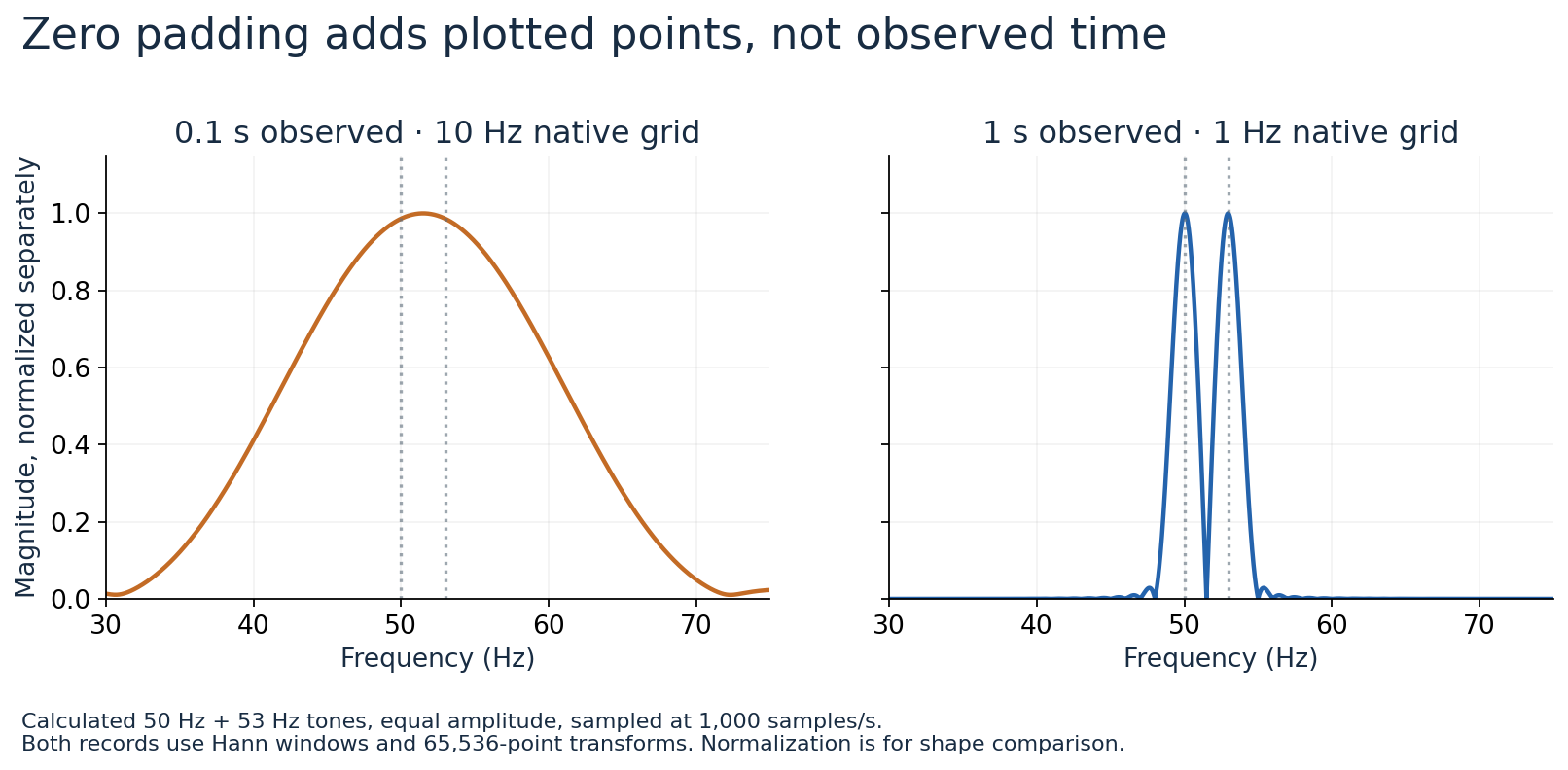
Figure 2. The same two tones, sampled at 1,000 samples per second, are analyzed with Hann windows. Dense zero padding makes both curves smooth. The one-second observation separates the tones clearly in this example; the 0.1-second observation does not. Vertical scales are normalized for comparison, not absolute amplitude measurement.

A specialized estimator using a strong prior model can sometimes estimate frequencies more precisely than a simple peak-spacing rule suggests. That does not invalidate the warning. It changes the assumptions supporting the estimate. I would ask whether the method assumes a known number of stationary sinusoids, how it behaves in noise, and whether those assumptions fit the incident. Numerical precision in an estimated frequency is not, by itself, a statement of measurement accuracy or evidence that two nearby physical sources were resolved.

The edges of a record become part of the analysis

The finite record has boundaries. If its beginning and end do not join smoothly under the periodic interpretation associated with the DFT, energy can appear across many bins rather than in one neat peak. This is often called spectral leakage. A tone at a frequency between our one-hertz grid points is an easy constructed example. The broader display does not necessarily mean the physical source suddenly began generating many unrelated tones. Some of that appearance follows from observing only a finite interval.

A window multiplies the record by a weighting sequence before transformation. Tapering the edges can reduce some leakage, while widening the main spectral feature and changing amplitude scaling. There is no free correction that makes every desirable property improve together. A window suited to revealing a weak tone near a strong one may be different from a choice suited to another measurement. I would document the window and its normalization beside the spectrum, because they are part of how the displayed evidence was produced.

For a stable sinusoid, amplitude correction commonly involves the sum of the window weights rather than blindly dividing by the original sample count. Noise-power estimates need a different accounting related to squared weights and effective bandwidth. SciPy's periodogram documentation distinguishes power spectral density from squared-magnitude spectrum and states their units.[4] The details are easy to overlook because both outputs can be drawn as a line against frequency. Identical-looking axes do not guarantee that the ordinates represent the same physical quantity.

A power density is not the power in one bin

Suppose a spectral-density estimate is expressed in volts squared per hertz. To estimate mean-square voltage over a frequency interval, integrate that density across the interval, using the estimator's conventions. A plotted height is not automatically the total contribution of that band. Changing frequency-bin width can change what a per-bin power display looks like even when the underlying noise process is unchanged. This is one reason screenshots without units and processing details are difficult to compare responsibly.

For a simple arithmetic illustration, imagine an ideal flat density of two square millivolts per hertz over a ten-hertz band. Its integrated mean-square contribution is twenty square millivolts. Over a five-hertz sub-band, it is ten. These values are constructed to make the units visible. They are not a prediction for a particular sensor. Taking the square root converts the mean-square quantity into an RMS voltage, provided the integration and one-sided or two-sided convention have been handled consistently.

One useful cross-check compares the appropriately integrated spectrum with the corresponding time-domain mean-square value. The transform's energy relationship provides the mathematical basis, but preprocessing must match: a removed mean, a taper, or an excluded band changes what is being compared. An apparent disagreement can reveal a normalization problem rather than a new physical effect. I would use a generated signal with a known amplitude to check the implementation before trusting an unexplained discrepancy in an expensive measurement.

A changing signal needs its order back

Return to the question that started the investigation: when did the disturbance begin? A whole-record spectrum combines contributions over the selected interval. To recover useful temporal context, we can examine successive short windows and arrange their spectra along a time axis. A spectrogram makes frequency content changing with time visible. Its appearance still depends on window duration, overlap, scaling, and color limits. The display is an analysis product with settings, not a photograph of frequency itself.

Short windows localize changes more closely in time but provide a broader spectral response. Longer windows can distinguish nearby steady components more clearly while mixing events over a longer interval. For our fifty- and fifty-three-hertz pair, a very short window is poorly suited to showing two separate tracks. For a brief impact, a long window can blur the timing we wanted to inspect. The useful choice follows from the question. One window cannot make every temporal and spectral distinction equally sharp.

Overlapping windows make the displayed evolution less discontinuous, but neighboring columns then share samples. A dense spectrogram should not be read as thousands of independent observations. If a detector counts consecutive bright columns as repeated evidence, that dependence matters. I would retain the original timestamps and investigate whether one event has simply appeared in many overlapping windows. This is a practical example of how a visualization decision can quietly become a statistical assumption further down the analysis pipeline.

Sampling is a separate limitation

At one thousand samples per second, an unqualified interpretation of arbitrarily high frequencies is impossible. Aliasing concerns how continuous-time content maps into the sampled record. Increasing the transform length afterward cannot repair ambiguity already introduced during acquisition. In the series article on the apparently backward wheel, we examined that problem directly. Here the distinction is enough: sampling rate limits which continuous-time distinctions the recording can support, while observation duration affects the detail available for analyzing the recorded sequence.

Doubling the sample rate while retaining the same one-second duration gives more samples and extends the representable frequency range under suitable acquisition conditions. It does not change the basic one-hertz DFT grid spacing for that duration. Doubling the duration at the original sample rate changes the grid spacing to half a hertz. These are different interventions. A request for “higher resolution” should specify which limitation matters before someone increases a setting that creates larger files without answering the actual question.

Missing or irregular timestamps complicate the ordinary recipe further. Feeding samples into a standard FFT as if they were uniformly spaced imposes a time model that may be false. Interpolation is itself a modeling step, and specialized methods exist for other sampling arrangements. I would first examine the acquisition record and identify gaps. A seemingly sophisticated spectral analysis cannot compensate for silently pretending that missing time never existed. The validity of its frequency axis depends on that assumption.

Use a known delay to test the phase interpretation

There is a useful distinction hidden in our first example. We changed the phase of only one component. That does not generally correspond to shifting the entire composite waveform in time. A delay of a whole recording changes each component's phase in proportion to its frequency. If an analysis labels every phase difference as one universal time delay, it needs to show that the different frequencies support the same delay, allowing for the ambiguity of complete cycles.

For a constructed delay of five milliseconds, a fifty-hertz component moves by one quarter of its cycle, or ninety degrees. A one-hundred-and-twenty-hertz component moves by six tenths of a cycle, or 216 degrees. The sign depends on the transform and comparison convention, but the proportional relationship is the point. A common delay produces different phase angles at different frequencies. Seeing equal phase angles at those two frequencies would not, by itself, establish that same five-millisecond delay.

Phase is also reported modulo a complete turn. A shift of 216 degrees can appear as minus 144 degrees on a display restricted to a particular angular range. The two describe the same position around the circle. Converting one isolated phase measurement into time therefore leaves whole-cycle ambiguity. Additional frequencies, a known timing range, or a recognizable event in the waveform can help resolve it. Without that information, an impressively precise delay estimate may hide several equally compatible possibilities.

This gives an independent way to challenge a proposed explanation. If a cable or processing stage is claimed to introduce an approximately constant delay across the relevant band, inspect whether its measured phase behavior is consistent with that model. If it is not, the response may be frequency dependent, the clocks may be misaligned, or the measurement may need correction. The calculation does not select among those explanations automatically. It tells us what a simple delay hypothesis should predict.

A quiet average can hide a brief disturbance

Imagine a ten-second constructed record containing a strong tone for only one tenth of a second. A second record contains a weaker tone continuously. Their whole-record energy in a selected band could be made equal by choosing the amplitudes appropriately. That does not make the underlying events equivalent. One could matter because of a brief overload, while the other could matter because of sustained exposure or interference. The appropriate interpretation depends on the phenomenon and the decision being made.

For an elementary energy calculation, take a unit-amplitude sinusoidal burst containing an integer number of cycles over 0.1 seconds, and zero values for the rest of a ten-second record. Ignoring any edge taper, its mean-square value over the full record is 0.005 in squared amplitude units. A continuous sinusoid with peak amplitude 0.1 has the same mean-square value. The burst's peak amplitude is ten times greater, even though the whole-record averages agree exactly under these assumptions.

The burst and continuous tone need not have identical detailed spectra, because switching the burst on and off spreads its spectral content. The example is about equal aggregate mean-square values, not identical Fourier coefficients. That qualification matters: a loose statement about “the same frequency result” would erase a distinction the calculation actually preserves. I would show the time trace beside the selected average and state the averaging interval, so the reader can distinguish a concentrated event from a persistent one.

For a real incident, the event's duration, clipping behavior, and timing relative to other system changes may be more useful than another decimal place in an average. I would retain a view that can answer those questions before reducing the recording to a summary. This is also why an analysis pipeline should preserve its inputs. A later investigator may need a different representation from the one that seemed sufficient when the first dashboard was designed.

Make the explanation survive a second view

For a fictional motor-vibration complaint, I would start by stating competing explanations: a persistent periodic component, an intermittent impact, a change in operating speed, or an acquisition artifact. Then I would choose views that distinguish them. The raw trace helps with clipping and timing; spectra help with repetition; a spectrogram helps with evolution. Correlation with independently recorded operating conditions may test a causal hypothesis. None of these views alone earns the right to name the failed component.

Reproducibility begins with the unprocessed record and the exact analysis choices. Preserve the sample rate, interval, units, calibration, window, detrending, transform length, normalization, and plotted range. Keep the script or calculation that produced the figure. Another person should be able to regenerate both the time trace and the spectrum and understand why they differ. A screenshot is useful for discussion, but it is a poor substitute for the evidence and processing history behind an important conclusion.

The strongest result here is not that frequency is better than time or that time is somehow more real. It is that each representation makes particular relationships easier to inspect. A full transform can preserve the finite record; a magnitude plot, an average, or a crop can conceal distinctions needed for a later question. I trust the analysis more when it can return to the original observation, explain its own assumptions, and show exactly which claim the available evidence supports.

References and method

1. SciPy, Discrete Fourier Transforms; transform definitions, normalization, and frequency indexing.
2. MIT OpenCourseWare, Lecture 9: Fourier Transform Properties; time shifts, phase, and transform properties.
3. MIT OpenCourseWare, The Discrete-Time Fourier Transform, Chapter 3; windowing and time-frequency resolution.
4. SciPy, Periodogram; spectral-density and spectrum scaling.

All plotted signals and numerical examples are constructed. The figures use explicit sinusoidal sums, uniformly spaced samples, NumPy Fourier transforms, and stated windows. They are not measurements from machinery or people. Sources checked on 3 October 2026.

Explore the complete Signals Around Us series.